11 October 2026·6 min read·machinelearning · datascience · mlinterview · python · scikitlearn · ai · codinginterview · deeplearning · dataengineering · learnmachinelearning

5 Mid-Tier ML Concepts You Should Know for Interviews

Bias and variance, L1 versus L2 regularisation, data leakage and honest cross validation, metrics for imbalanced data, and gradient descent: the questions that come after "name an algorithm".

After "name an algorithm"

The first ML interview question is usually some version of "what would you use for this". The second one is where it gets interesting: "it overfit, what do you do", "why did it look great offline and fail in production", "your fraud model is 99% accurate, is that good". Those are diagnosis questions, and they're built on five concepts.

I've hit every one of these on real models. Each section has the idea, why it matters, code I ran before posting (scikit-learn 1.7, numpy 2.2), and the trap. Save it and come back the night before.

5 mid tier ML concepts

A 36 second version of this article

The five concepts in under 40 seconds, captions on.

Poster frame of the explainer video: Your model is 99% accurate. it is also useless. — The five concepts in under 40 seconds, captions on. Watch the video: https://designsbyduhart.org/blog/5-mid-tier-ml-concepts-for-interviews/

1. Bias versus variance

A model's expected error on new data splits into three parts: bias, variance and irreducible noise. Bias is error from the model being too simple to capture the pattern (a straight line through a curve). Variance is error from the model being too sensitive to the particular training sample (a deep tree that changes completely when you add ten rows). Noise is the part no model can remove. Making a model more flexible usually lowers bias and raises variance, which is the tradeoff.

The practical value is diagnosis. Plot a learning curve: training and validation score as the training set grows.

Both scores low and close together: high bias. More data won't help. Use a more expressive model, add features, or reduce regularisation.
Training score high, validation much lower, a big gap: high variance. More data helps, and so do regularisation, a simpler model, or bagging.

Bias versus variance

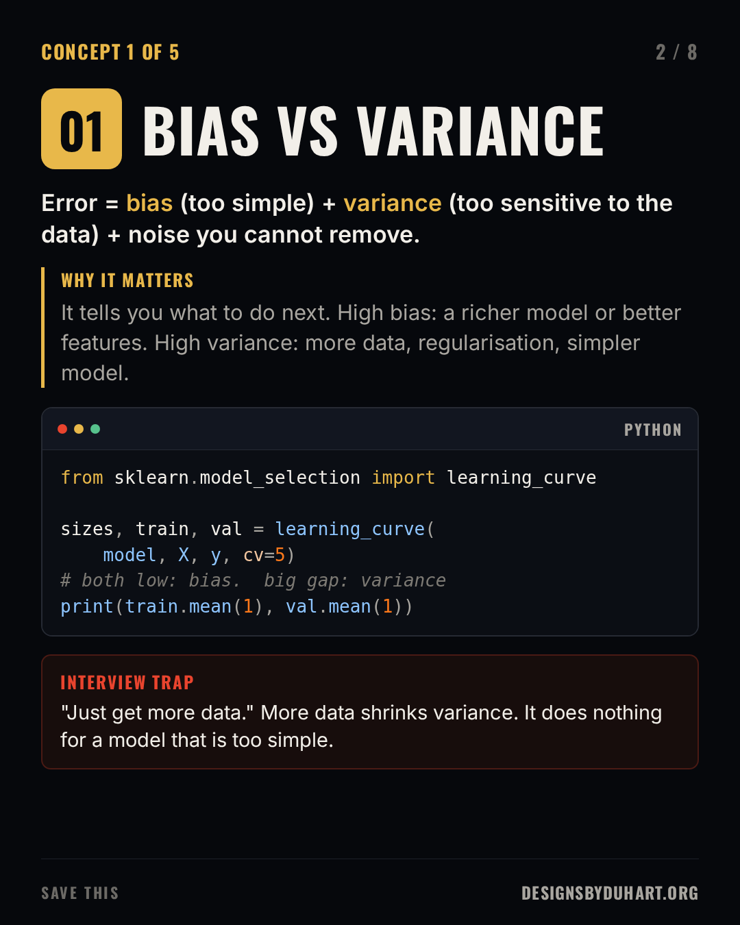
Slide 2 of 8: BIAS VS VARIANCE. Error = bias (too simple) + variance (too sensitive to the data) + noise you cannot remove. Why it matters: It tells you what to do next. High bias: a richer model or better features. High variance: more data, regularisation, simpler model. A code card (python) shows: from sklearn.model_selection import learning_curve sizes, train, val = learning_curve( model, X, y, cv=5) # both low: bias. big gap: variance print(train.mean(1), val.mean(1)) Interview trap: "Just get more data." More data shrinks variance. It does nothing for a model that is too simple. — Read the learning curve before you change anything.

A learning curve for a deliberately overfit tree: training accuracy near 1.0, validation well below. That gap is variance.

python

from sklearn.datasets import make_classification
from sklearn.model_selection import learning_curve
from sklearn.tree import DecisionTreeClassifier

X, y = make_classification(n_samples=1500, n_features=20, n_informative=5, flip_y=0.1, random_state=0)
sizes, train, val = learning_curve(DecisionTreeClassifier(random_state=0), X, y, cv=5,
                                   train_sizes=[0.1, 0.4, 1.0])
for n, t, v in zip(sizes, train.mean(1), val.mean(1)):
    print(f"{n:5d} rows  train {t:.2f}  val {v:.2f}")

The trap: "get more data" is the reflexive answer, and it only works for variance. A high bias model given ten times the data stays exactly as wrong.

2. L1 versus L2 regularisation

Regularisation adds a penalty on the size of the weights to the loss, so the model trades a little training fit for simpler weights that generalise better.

L2 (Ridge) penalises the sum of squared weights. It shrinks every weight toward zero smoothly and rarely makes any exactly zero. With correlated features it spreads weight across them instead of picking one arbitrarily.
L1 (Lasso) penalises the sum of absolute weights. Its geometry (the corners of the diamond shaped constraint) drives some weights to exactly zero, so it performs feature selection as a side effect.
Elastic net mixes both, which helps when you want sparsity but have groups of correlated features.

L1 versus L2

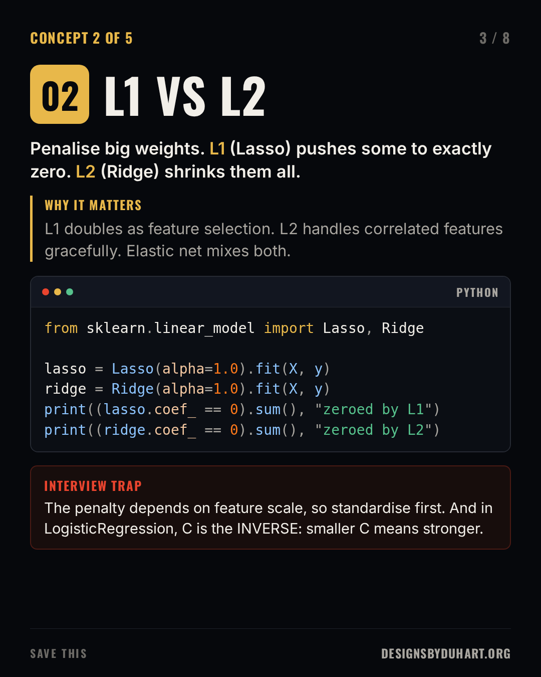
Slide 3 of 8: L1 VS L2. Penalise big weights. L1 (Lasso) pushes some to exactly zero. L2 (Ridge) shrinks them all. Why it matters: L1 doubles as feature selection. L2 handles correlated features gracefully. Elastic net mixes both. A code card (python) shows: from sklearn.linear_model import Lasso, Ridge lasso = Lasso(alpha=1.0).fit(X, y) ridge = Ridge(alpha=1.0).fit(X, y) print((lasso.coef_ == 0).sum(), "zeroed by L1") print((ridge.coef_ == 0).sum(), "zeroed by L2") Interview trap: The penalty depends on feature scale, so standardise first. And in LogisticRegression, C is the INVERSE: smaller C means stronger. — L1 zeroes weights out; L2 shrinks them all.

On data where only 5 of 30 features matter, Lasso zeroes most of the useless ones; Ridge zeroes none.

python

from sklearn.datasets import make_regression
from sklearn.linear_model import Lasso, Ridge

X, y = make_regression(n_samples=500, n_features=30, n_informative=5, noise=10, random_state=0)
lasso = Lasso(alpha=1.0).fit(X, y)
ridge = Ridge(alpha=1.0).fit(X, y)
print((lasso.coef_ == 0).sum(), "of 30 weights zeroed by L1")
print((ridge.coef_ == 0).sum(), "of 30 weights zeroed by L2")

The traps: the penalty is on raw weight size, so a feature measured in thousands gets penalised differently from one measured in fractions. Standardise first. And watch the parameter direction: alpha in Ridge and Lasso is the penalty strength, but C in LogisticRegression and SVMs is its inverse, so a smaller C means more regularisation. People get that backwards in interviews constantly.

3. Data leakage and honest cross validation

Leakage is any path by which information that wouldn't be available at prediction time gets into training. The model looks brilliant in validation and disappoints in production, and it's the most common reason I've seen an offline score not survive contact with real traffic.

The usual suspects:

Preprocessing leakage. Fitting a scaler, an imputer or a feature selector on the whole dataset before splitting. The training folds have now seen statistics of the validation fold. The fix is a Pipeline, so every step is fit inside each training fold only.
Target leakage. A feature that's a consequence of the label. "Refund issued" predicts churn wonderfully, because it happens after the customer complained.
Time leakage. Shuffling time series, so the model trains on next week to predict last week. Use TimeSeriesSplit or a strict cutoff date.
Group leakage. The same user, patient or device in both train and test, so the model recognises the entity instead of learning the pattern. Use GroupKFold.

Data leakage

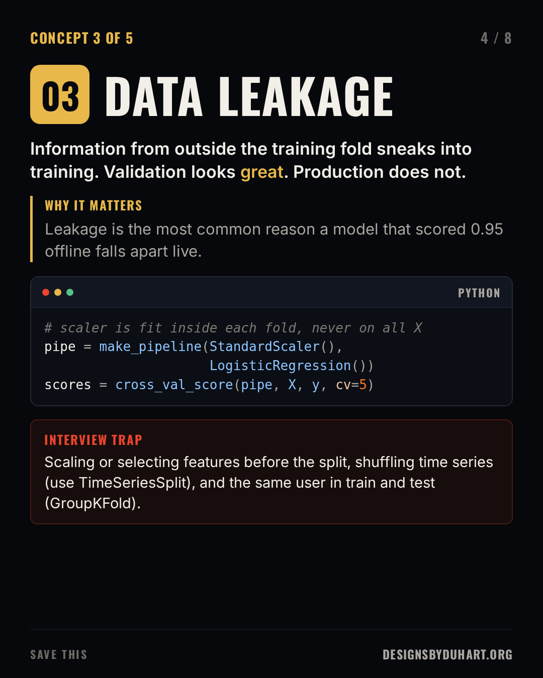
The pipeline version is the honest one: the scaler and the selector are refit on each training fold, never on the rows they are scored on.

python

from sklearn.datasets import make_classification
from sklearn.feature_selection import SelectKBest
from sklearn.linear_model import LogisticRegression
from sklearn.model_selection import cross_val_score
from sklearn.pipeline import make_pipeline
from sklearn.preprocessing import StandardScaler

X, y = make_classification(n_samples=300, n_features=2000, n_informative=5, random_state=0)

# leaky: feature selection saw every row, including the ones used for scoring
X_sel = SelectKBest(k=20).fit_transform(X, y)
leaky = cross_val_score(LogisticRegression(max_iter=1000), X_sel, y, cv=5).mean()

# honest: selection happens inside each training fold
pipe = make_pipeline(StandardScaler(), SelectKBest(k=20), LogisticRegression(max_iter=1000))
honest = cross_val_score(pipe, X, y, cv=5).mean()
print(f"leaky {leaky:.2f}  honest {honest:.2f}")

With many features and few rows, the leaky score comes out noticeably higher than the honest one, for a model that is exactly the same. That gap is the leakage.

4. Imbalanced data: 99% accurate, 100% useless

If 1% of transactions are fraud, a model that always answers "not fraud" is 99% accurate and catches nothing. Accuracy is the wrong question when classes are imbalanced. Better ones:

Precision: of everything you flagged, what fraction was really fraud? Low precision means analysts wading through false alarms.
Recall: of all the fraud that happened, what fraction did you catch? Low recall means losses.
F1 combines the two into one number, the harmonic mean.
PR-AUC (average precision) summarises precision and recall across every threshold.

The threshold is a business decision, not a default. 0.5 is arbitrary; choose it from the cost of a false alarm against the cost of a miss. class_weight="balanced" tells many scikit-learn models to weigh the rare class more during training.

Metrics for imbalanced data

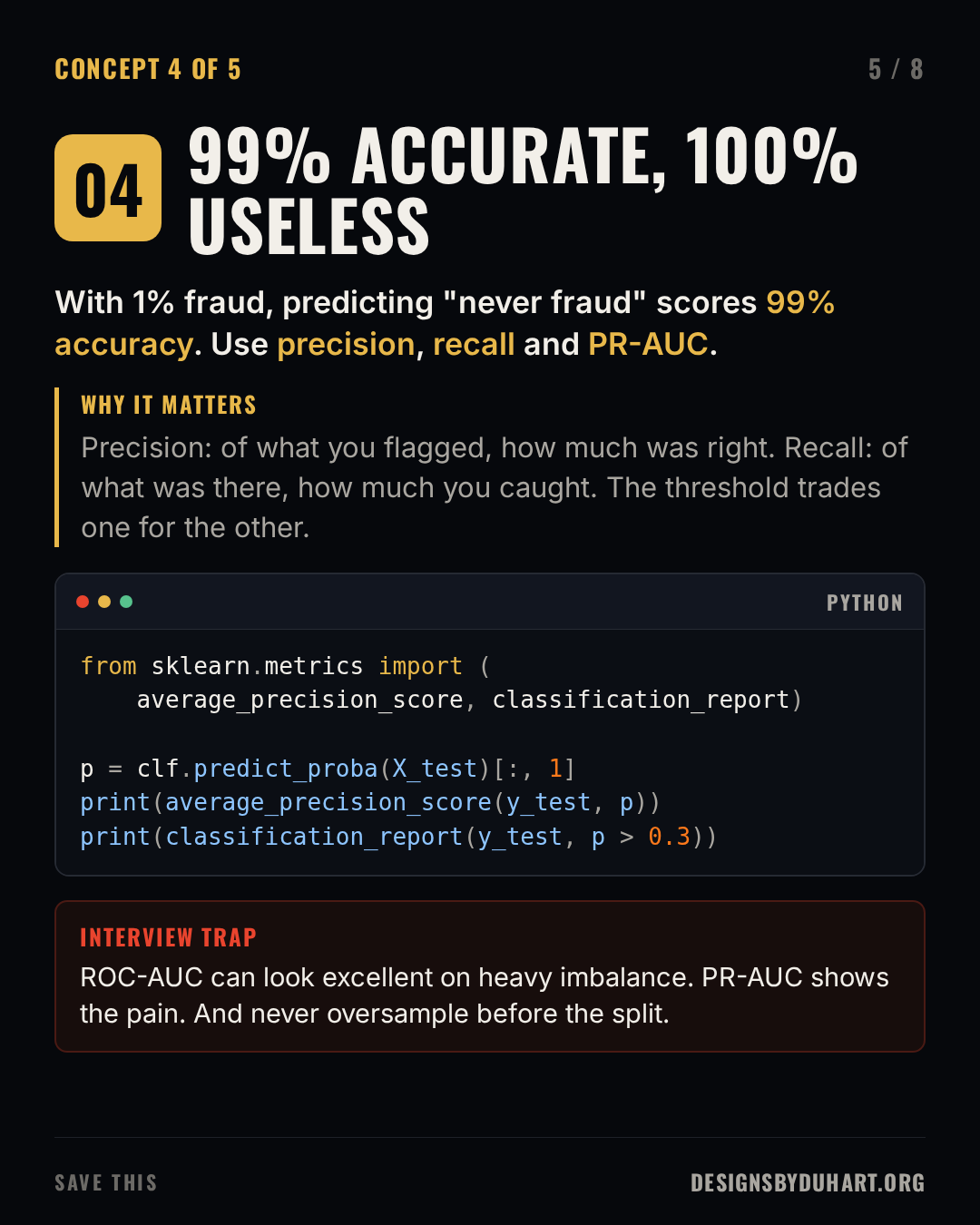
Slide 5 of 8: 99% ACCURATE, 100% USELESS. With 1% fraud, predicting "never fraud" scores 99% accuracy. Use precision, recall and PR-AUC. Why it matters: Precision: of what you flagged, how much was right. Recall: of what was there, how much you caught. The threshold trades one for the other. A code card (python) shows: from sklearn.metrics import ( average_precision_score, classification_report) p = clf.predict_proba(X_test)[:, 1] print(average_precision_score(y_test, p)) print(classification_report(y_test, p > 0.3)) Interview trap: ROC-AUC can look excellent on heavy imbalance. PR-AUC shows the pain. And never oversample before the split. — Precision, recall, PR-AUC and a threshold you chose on purpose.

A 1% positive class. The always-negative baseline is 99% accurate with zero recall; the model is judged on average precision and a chosen threshold instead.

python

from sklearn.datasets import make_classification
from sklearn.dummy import DummyClassifier
from sklearn.linear_model import LogisticRegression
from sklearn.metrics import accuracy_score, average_precision_score, recall_score
from sklearn.model_selection import train_test_split

X, y = make_classification(n_samples=20000, weights=[0.99], flip_y=0, random_state=0)
X_tr, X_te, y_tr, y_te = train_test_split(X, y, stratify=y, random_state=0)

dummy = DummyClassifier(strategy="most_frequent").fit(X_tr, y_tr)
print("dummy accuracy", accuracy_score(y_te, dummy.predict(X_te)),
      "recall", recall_score(y_te, dummy.predict(X_te)))

clf = LogisticRegression(class_weight="balanced", max_iter=1000).fit(X_tr, y_tr)
p = clf.predict_proba(X_te)[:, 1]
print("PR-AUC", round(average_precision_score(y_te, p), 3))
for t in (0.5, 0.8, 0.95):
    print(t, "recall", round(recall_score(y_te, p > t), 2))

The traps. ROC-AUC can look excellent on heavily imbalanced data because the huge number of true negatives keeps the false positive rate tiny; Saito and Rehmsmeier (PLOS ONE, 2015) showed the precision recall plot is more informative in exactly that setting. And if you oversample (SMOTE or plain duplication), do it inside the training fold only. Oversampling before the split copies minority rows into the test set, which is leakage again.

5. Gradient descent

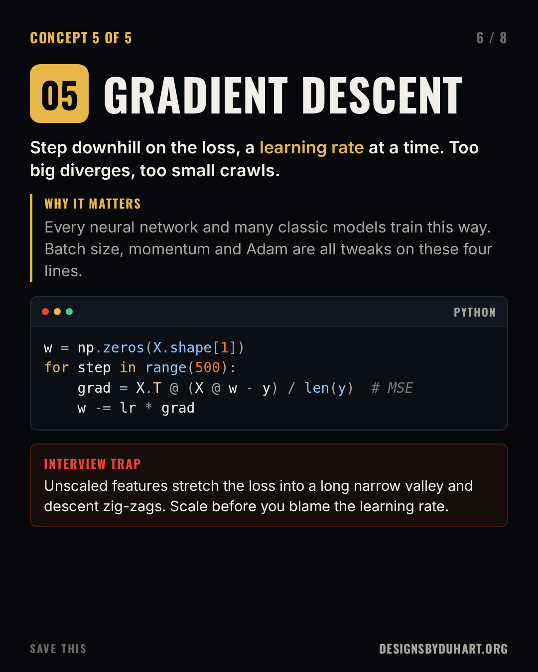
Most models with a differentiable loss are trained the same way: compute the gradient of the loss with respect to the weights, take a step in the opposite direction, repeat. The learning rate is the step size. Too large and the loss bounces around or diverges; too small and training crawls or stalls.

The variants are about how much data each step sees. Batch gradient descent uses the whole dataset per step (stable, expensive). Stochastic uses one example (cheap, noisy). Mini-batch, the default in deep learning, uses a few dozen to a few thousand. Momentum and Adam smooth the noisy steps and adapt the step size per weight.

Gradient descent

Watch the learning rate

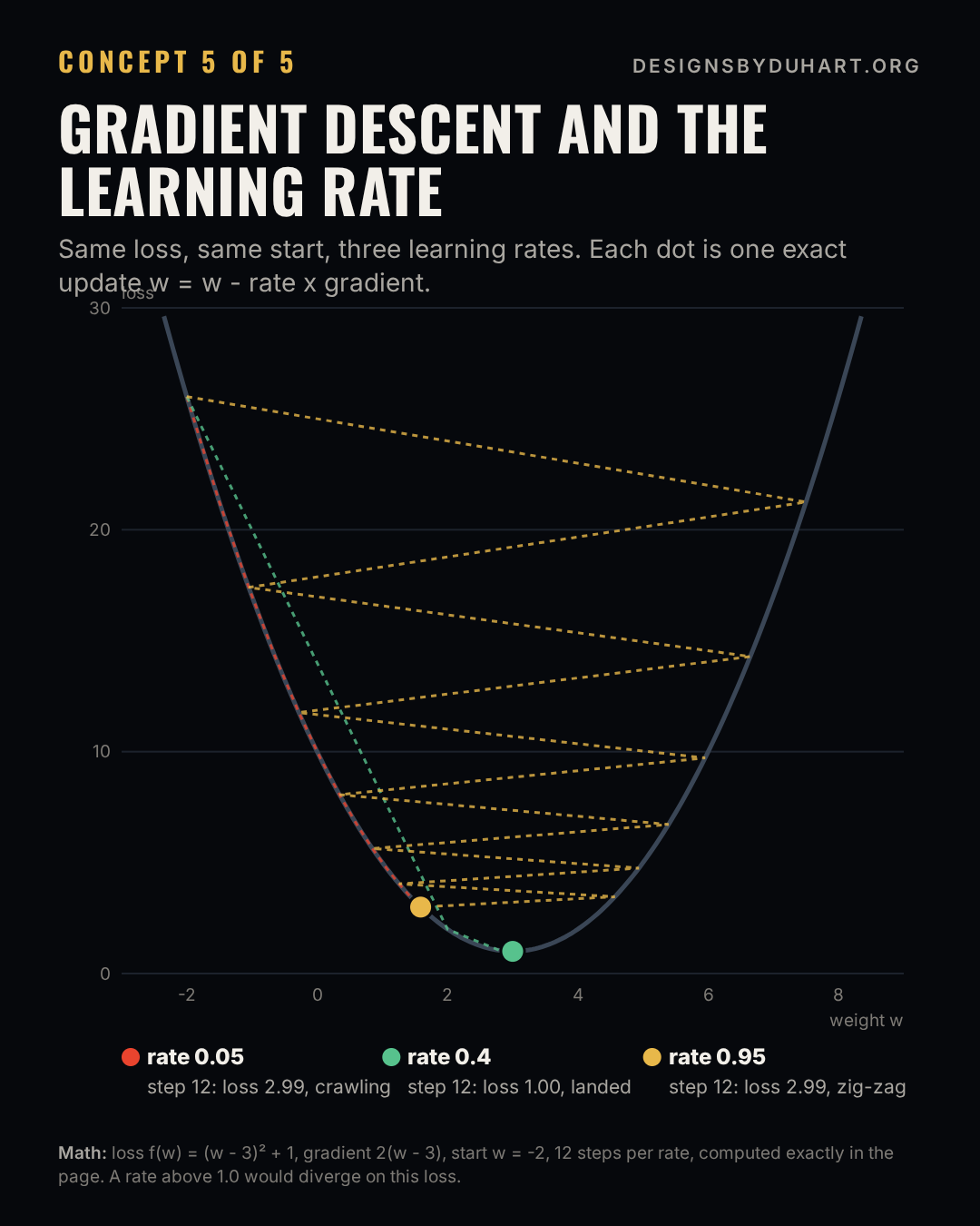
Twelve exact steps for each rate. Too small crawls, too big zig-zags, the right one lands fast.

Final frame of the animated chart. Animation of gradient descent on the loss (w - 3) squared plus 1, starting at w = -2: a learning rate of 0.05 crawls down the slope, 0.4 reaches the minimum in a few steps, and 0.95 zig-zags across the valley. — Twelve exact steps for each rate. Too small crawls, too big zig-zags, the right one lands fast. Watch the video: https://designsbyduhart.org/blog/5-mid-tier-ml-concepts-for-interviews/

Plain batch gradient descent for linear regression with numpy. On standardised features it converges; feed it raw features with wildly different scales and the same learning rate blows up.

python

import numpy as np

rng = np.random.default_rng(0)
X = rng.normal(size=(1000, 3)) * [1.0, 50.0, 0.01]      # three very different scales
y = X @ np.array([2.0, 0.1, 300.0]) + rng.normal(size=1000)

def fit(X, y, lr, steps=500):
    w = np.zeros(X.shape[1])
    for _ in range(steps):
        grad = X.T @ (X @ w - y) / len(y)   # gradient of mean squared error / 2
        w -= lr * grad
    return np.mean((X @ w - y) ** 2)

Xs = (X - X.mean(0)) / X.std(0)
print("scaled   MSE", round(fit(Xs, y, lr=0.1), 2))
with np.errstate(over="ignore", invalid="ignore"):
    print("unscaled MSE", fit(X, y, lr=0.1))     # diverges: inf or nan

The trap: when descent zig-zags or diverges, people reach for the learning rate first. Often the real problem is that features on very different scales stretch the loss surface into a long, narrow valley, so any single step size is too big in one direction and too small in another. Standardise the features and the same learning rate behaves.

The one line answers

If you remember nothing else, remember these. They're the slide I'd want in my pocket walking into the room.

The one line answers

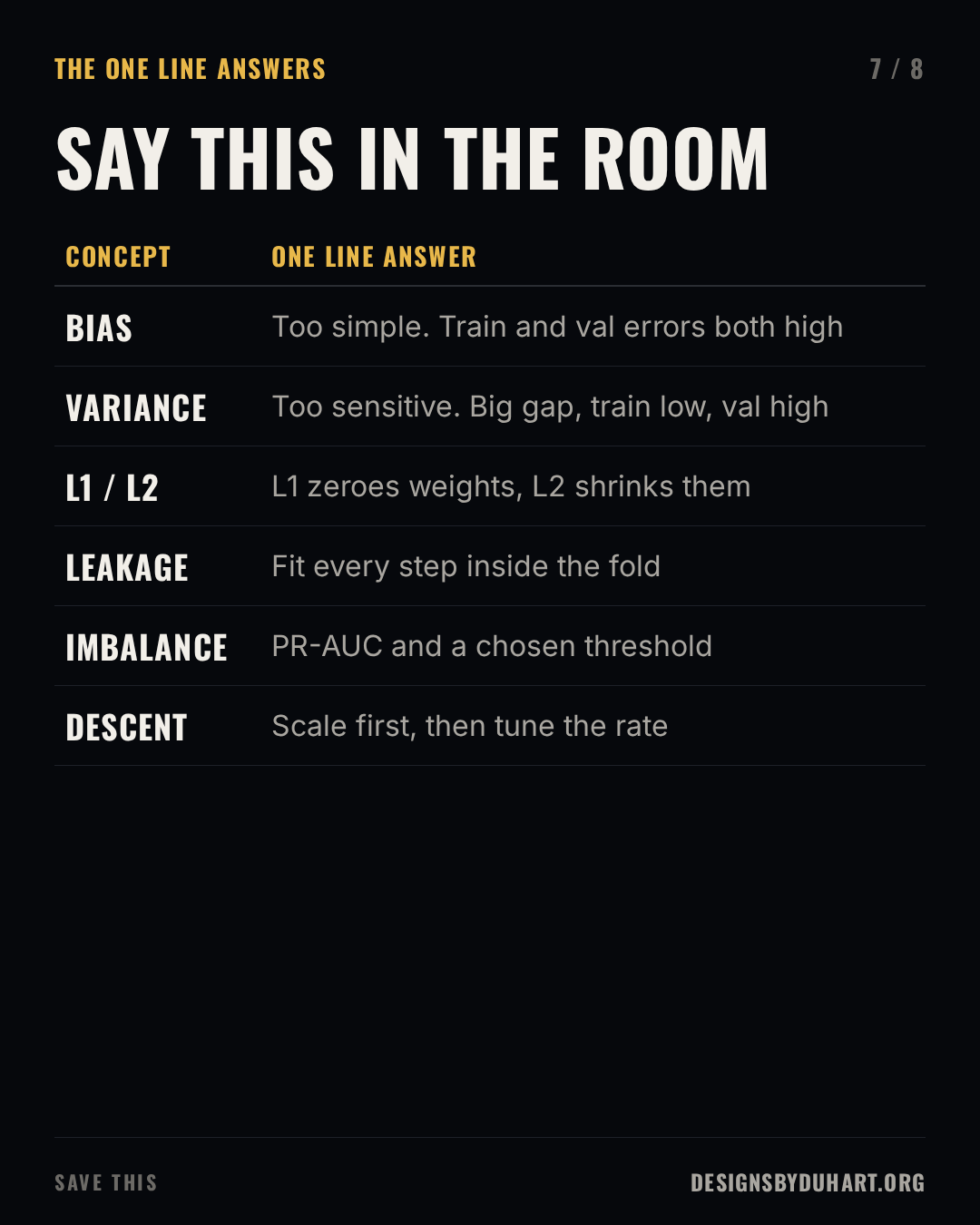
Slide 7 of 8: SAY THIS IN THE ROOM. A table: CONCEPT, ONE LINE ANSWER; BIAS, Too simple. Train and val errors both high; VARIANCE, Too sensitive. Big gap, train low, val high; L1 / L2, L1 zeroes weights, L2 shrinks them; LEAKAGE, Fit every step inside the fold; IMBALANCE, PR-AUC and a chosen threshold; DESCENT, Scale first, then tune the rate. — Bias, variance, L1 and L2, leakage, imbalance and descent in one table.

Every one of these is about the same habit: diagnose before you tune. Read the learning curve, keep the validation honest, choose the metric that matches the problem, and fix the data before you blame the optimiser.

Next in the series: CI/CD pipelines, and the GitLab CI file I'd show in an interview.

Save it for your next interview

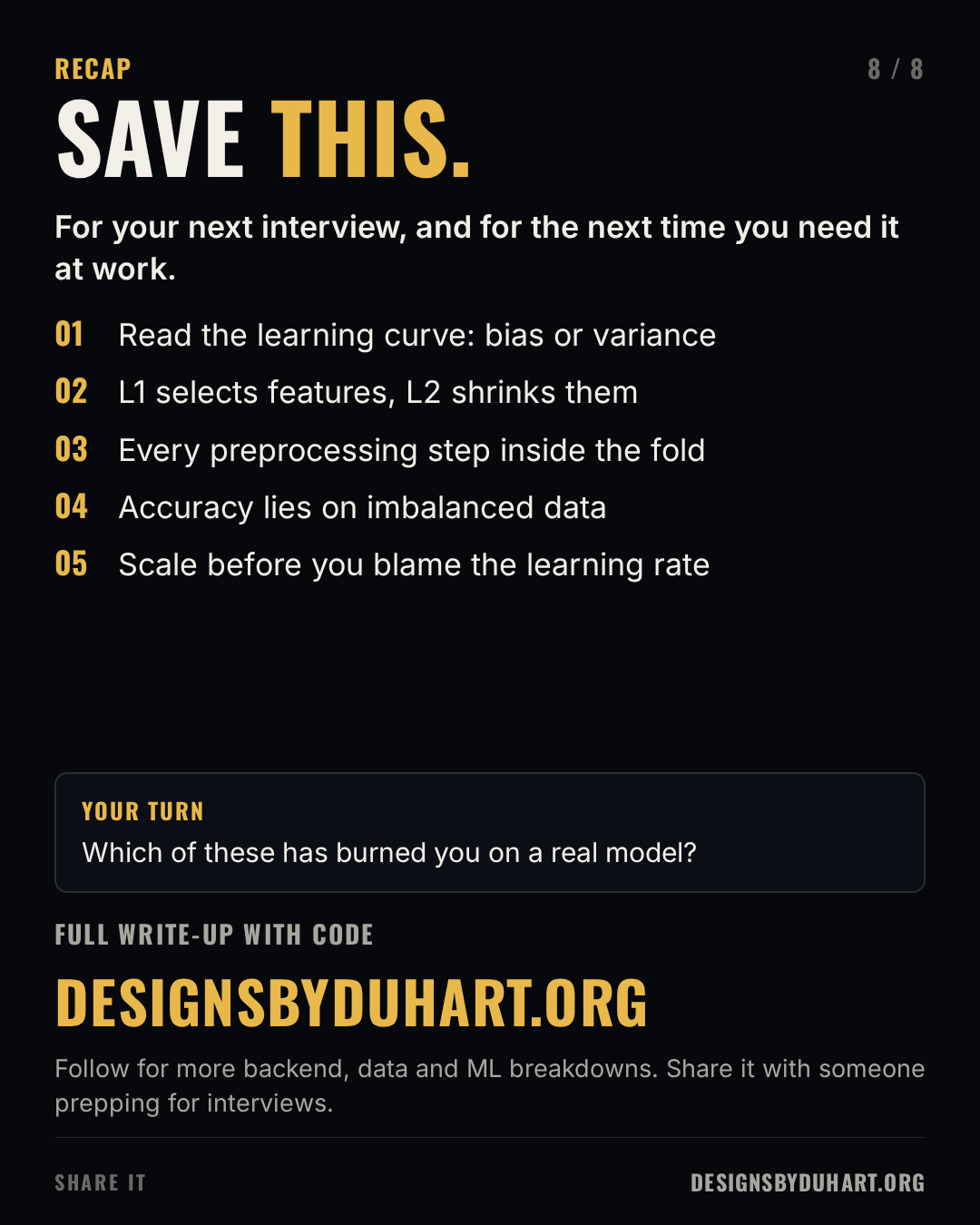
Closing slide 8 of 8: Save this. Recap: Read the learning curve: bias or variance; L1 selects features, L2 shrinks them; Every preprocessing step inside the fold; Accuracy lies on imbalanced data; Scale before you blame the learning rate. Your turn: Which of these has burned you on a real model? Full write-up with code at designsbyduhart.org. — The recap card.

Next in the interview series: CI/CD pipelines, and the GitLab CI file I would show in an interview.

More: LinkedIn · Instagram. Portfolio and case studies: designsbyduhart.org.

If any of this saved you an afternoon, Buy me a coffee.