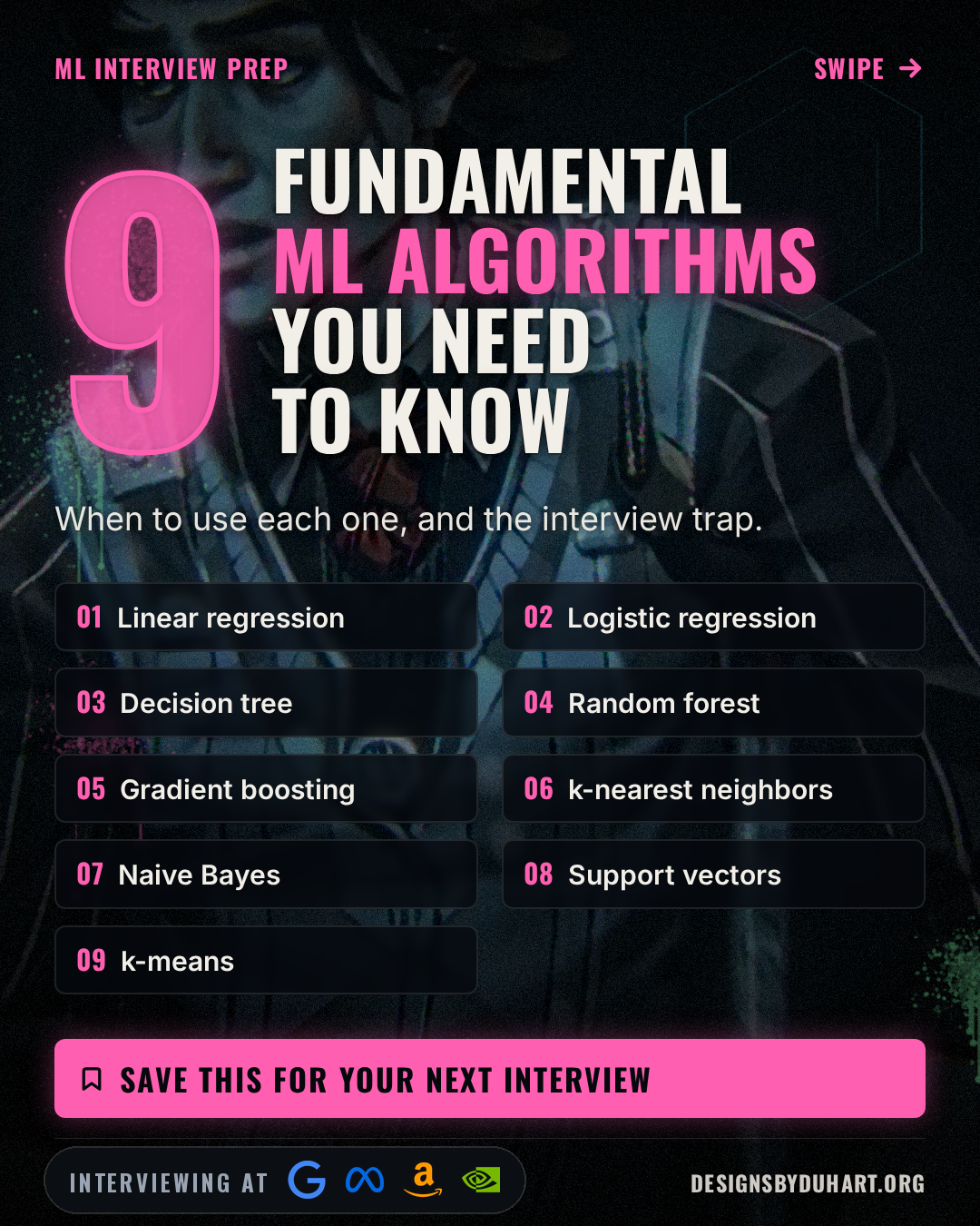
9 Fundamental ML Algorithms You Need to Know
Linear and logistic regression, decision trees, random forests, gradient boosting, k-NN, Naive Bayes, SVMs and k-means: what each does, when to reach for it, and the interview trap, with scikit-learn code.
The toolbox before the deep end
Every few months somebody declares the classical algorithms dead, and every few months I go back to work and use them. Deep learning owns images, audio and language. On the tables most companies actually run on (users, orders, events, transactions) these nine still do most of the work, and they're what you get asked about in ML and data interviews.
For each one: the family it belongs to, what it does in a sentence, when I'd reach for it, a scikit-learn snippet (I ran every one of them against scikit-learn 1.7 before posting), and the trap that catches people. The carousel slides are in here too, so you can save the article and skim.
9 fundamental ML algorithms
The 38 second version
1. Linear regression
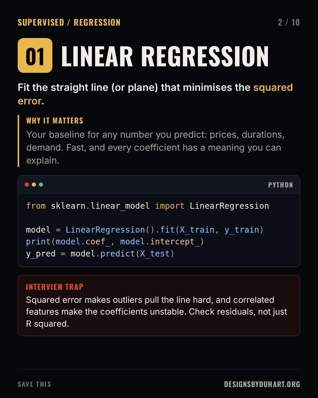
Linear regression predicts a number as a weighted sum of the features plus an intercept, choosing the weights that minimise the sum of squared errors. There's a closed form solution, it trains in milliseconds, and each coefficient tells you how much the prediction moves per unit of that feature, holding the rest fixed.
Use it as the baseline for any continuous target. If a fancier model can't beat it by a margin you care about, ship the line.
The traps are all about assumptions. Squaring the errors means one outlier with a huge residual pulls the whole fit toward it. Strongly correlated features (multicollinearity) let the coefficients swing wildly between fits while predictions barely change, which matters the moment someone wants to read the coefficients as explanations. And a good R squared doesn't mean a good model: plot the residuals against the predictions. A pattern there means the relationship isn't linear. Ridge (L2) and Lasso (L1) regression are the regularised versions, and they're the next question.
Linear regression
2. Logistic regression
Logistic regression takes the same weighted sum and passes it through the sigmoid function, which maps any number to a probability between 0 and 1. It's trained by minimising log loss (cross entropy), which punishes confident wrong answers hard. Threshold the probability (0.5 by default, but you should choose it) and you have a classifier.
It's the first model I'd fit for any yes or no question. It's fast, it's well calibrated out of the box compared with most models, and its coefficients are log odds you can explain to a product manager.
Two traps. The name: it's a classification algorithm, and interviewers do ask. And the defaults: scikit-learn's LogisticRegression applies L2 regularisation with C=1.0 unless you say otherwise, so features on very different scales get penalised unevenly. Put a StandardScaler in front of it.
Logistic regression
![Slide 3 of 10: LOGISTIC REGRESSION. A linear score squeezed through a sigmoid into a probability, trained with log loss. Why it matters: The default first model for yes or no questions: churn, fraud, click. Gives probabilities and coefficients you can read. A code card (python) shows: from sklearn.linear_model import LogisticRegression clf = LogisticRegression(C=1.0).fit(X_train, y_train) p = clf.predict_proba(X_test)[:, 1] Interview trap: Despite the name, it is a classifier. And scikit-learn regularises it by default (L2, C=1.0), so scale your features.](https://media.designsbyduhart.org/viral/bbb82e8b9dfcfaf8.png)
3. Decision tree
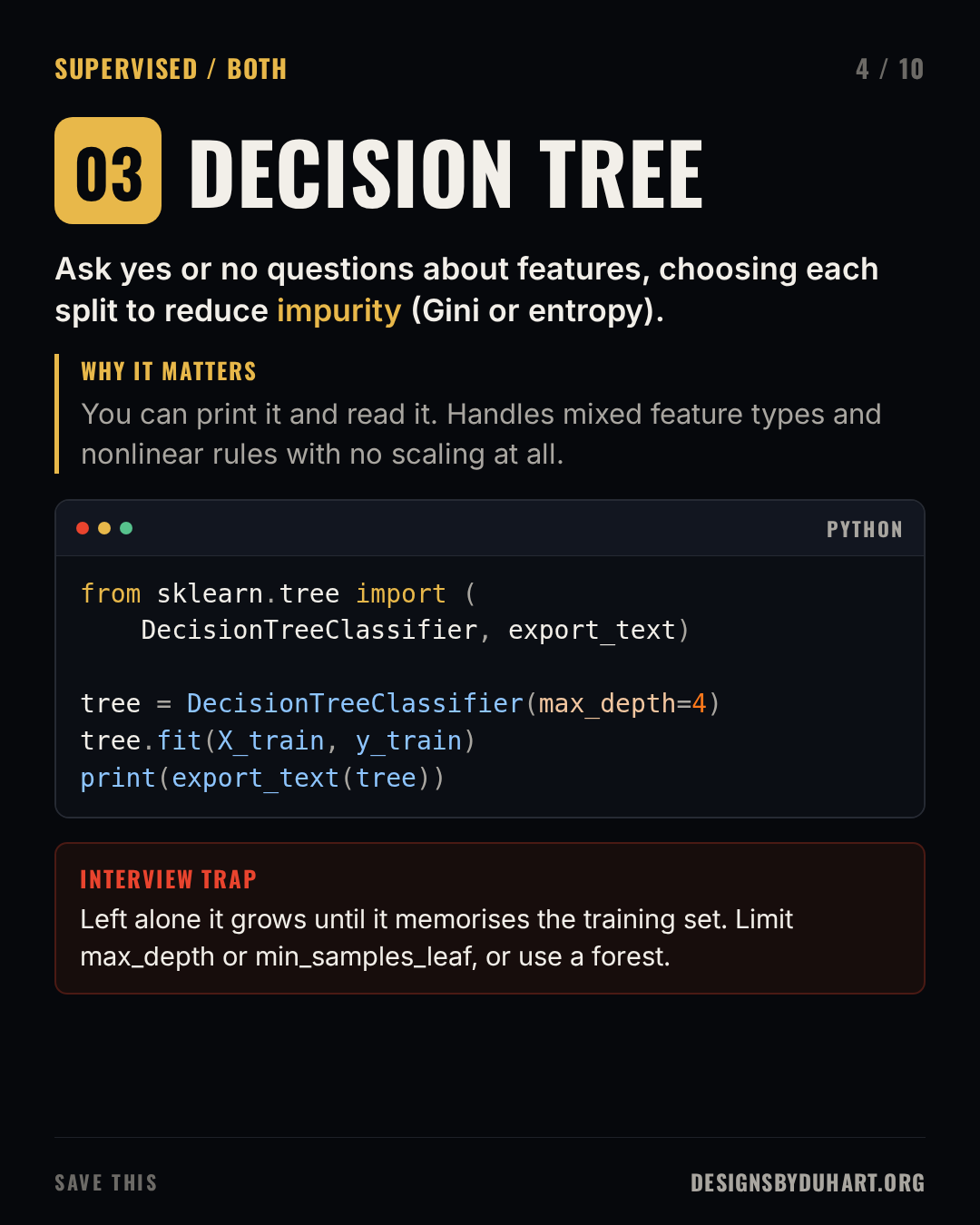
A decision tree learns a flowchart. At each node it picks the feature and threshold that best separate the targets, measured by impurity (Gini or entropy for classification, squared error for regression), then repeats on each side. Prediction is walking from the root to a leaf.
Trees need no feature scaling, handle nonlinear rules and interactions naturally, and you can print one and read it, which is rare in machine learning.
Their weakness is variance. An unconstrained tree keeps splitting until every leaf is pure, which means it memorises the training set, noise included, and a small change in the data can produce a completely different tree. Limit max_depth, min_samples_leaf or use cost complexity pruning. In practice the bigger fix is not to use one tree at all, which is what the next two algorithms do.
Decision tree
4. Random forest
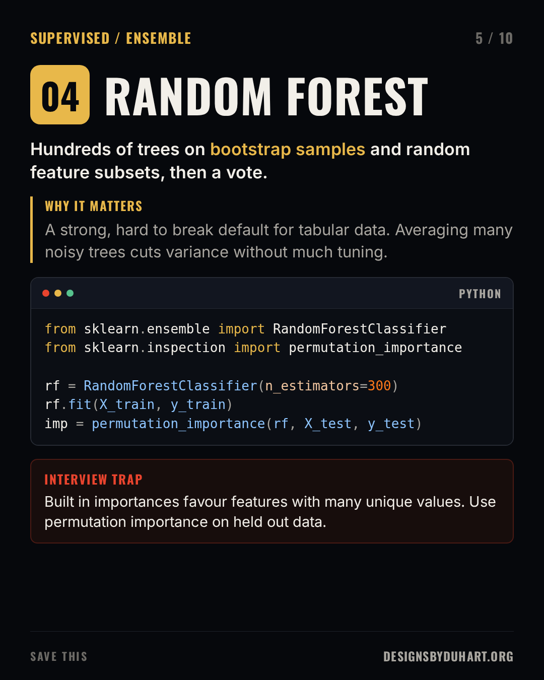
A random forest (Breiman, 2001) trains hundreds of decision trees, each on a bootstrap sample of the rows (sampling with replacement) and each split considering only a random subset of the features. Then it averages their predictions or takes a vote. Each tree overfits in its own way, and averaging many decorrelated, overfit trees cancels much of that variance. That's bagging plus feature randomness.
It's one of the hardest models to get badly wrong: little tuning, robust to outliers and irrelevant features, and you get an out of bag error estimate for free.
The trap is feature importance. The default feature_importances_ (mean decrease in impurity) is computed on training data and is biased toward features with many unique values, like IDs and continuous columns. A random ID column can look important. Use permutation importance on a held out set instead: shuffle one feature and measure how much the score drops.
Random forest
5. Gradient boosting
Gradient boosting (Friedman, 2001) also builds an ensemble of trees, but in sequence. Each new, shallow tree is fit to the errors the current ensemble still makes (more precisely, to the negative gradient of the loss), and its prediction is added in with a small learning rate. Many weak learners, each correcting the last.
This is the family behind XGBoost, LightGBM and CatBoost, and scikit-learn's HistGradientBoostingClassifier is a fast implementation of the same idea. On typical tabular data it is often the strongest model available. A NeurIPS 2022 benchmark by Grinsztajn, Oyallon and Varoquaux found tree based models like XGBoost and random forests still outperformed deep learning models on medium sized tabular datasets. If I have a table and a target, a boosted model is usually the second thing I fit, after the linear baseline.
Gradient boosting
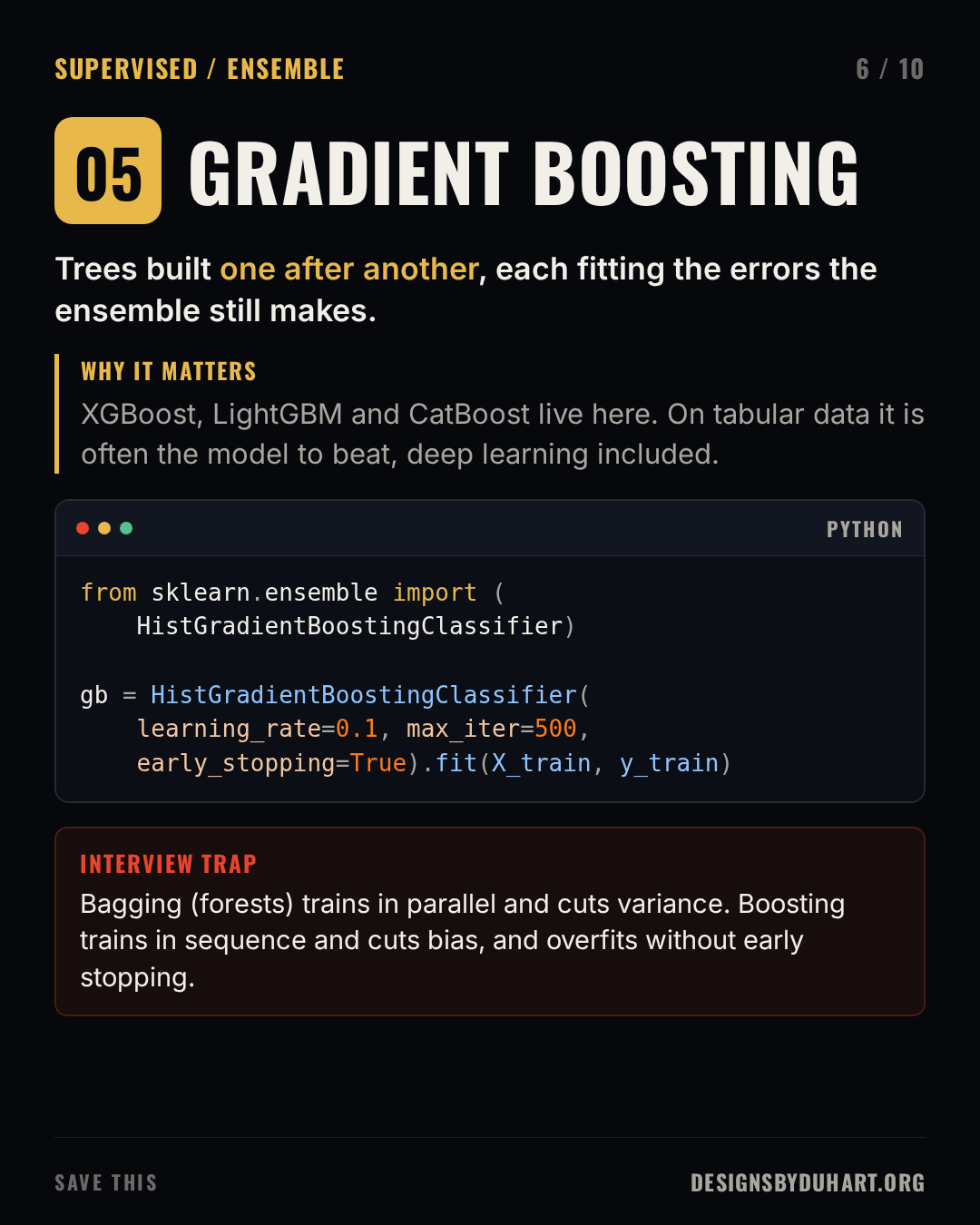
The classic interview question is bagging versus boosting. Bagging (random forests) trains independent models in parallel on resampled data and averages them, which mainly reduces variance. Boosting trains models in sequence, each focusing on the previous errors, which mainly reduces bias. Because boosting keeps fitting the residuals, it will eventually fit the noise too, so the number of rounds matters: use early stopping on a validation set and a small learning rate.
6. k-nearest neighbors
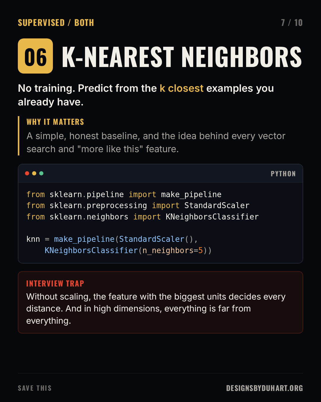
k-NN doesn't really train. It stores the training data, and to predict, finds the k closest examples (usually by Euclidean distance) and takes a majority vote, or the average for regression. Small k gives a jagged, high variance boundary; large k smooths it out.
It's a useful baseline, and the idea is everywhere: "more like this" recommendations and vector search over embeddings are nearest neighbour lookups, just with approximate indexes so they scale.
The traps are distance and dimension. If one feature is income in dollars and another is age in years, income decides every distance unless you scale. And as dimensions grow, distances between points become more and more similar to each other (the curse of dimensionality), so "nearest" stops meaning much. Prediction cost also grows with the training set, since every query compares against stored points unless you use an index.
k-nearest neighbors
7. Naive Bayes
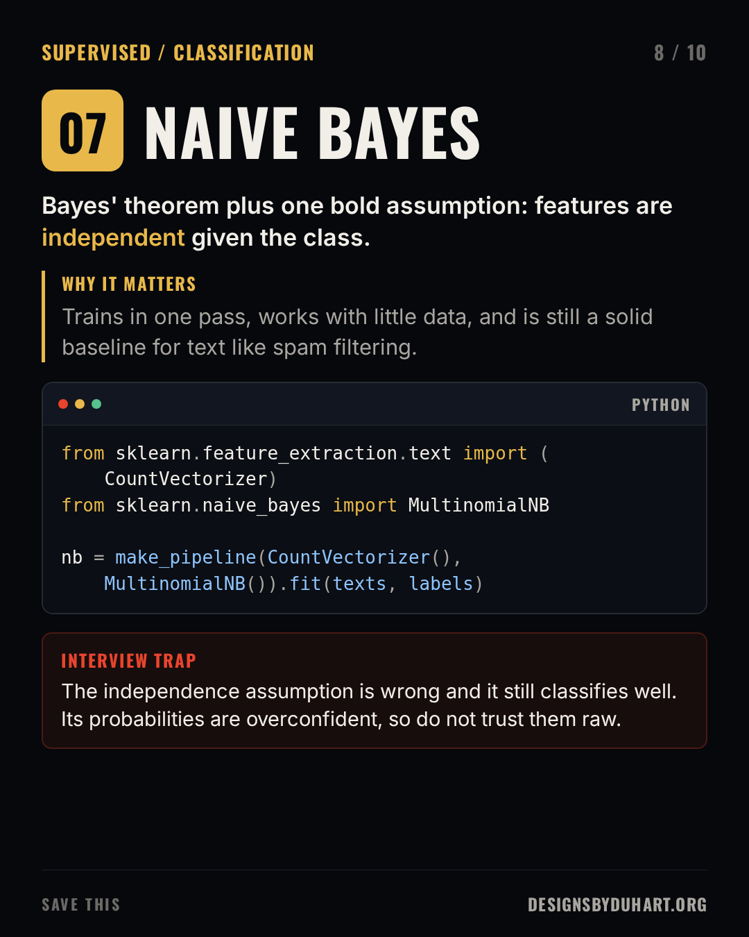
Naive Bayes applies Bayes' theorem to get the probability of each class given the features, with one simplifying assumption: the features are independent of each other once you know the class. That assumption makes the maths trivial, so training is a single pass of counting.
The assumption is almost always false (in an email, "cash" and "prize" are clearly not independent), and it still classifies surprisingly well, because getting the ranking of classes right doesn't need the probabilities to be right. It's quick to train, works with little data, and is still a respectable baseline for text classification. Multinomial Naive Bayes on word counts is the textbook spam filter.
The trap: those probabilities are usually overconfident, pushed toward 0 and 1, precisely because correlated evidence gets counted as if it were independent. Use the ranking, and calibrate before you use the numbers.
Naive Bayes
8. Support vector machine
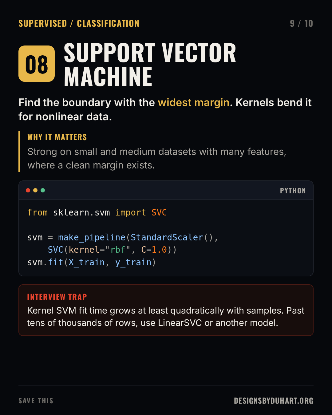
A support vector machine finds the boundary between classes with the widest possible margin to the nearest points on each side, the support vectors. C trades margin width against training errors. The kernel trick lets it fit nonlinear boundaries (the RBF kernel is the usual default) by computing similarities as if the data were mapped into a higher dimensional space, without ever building that space.
SVMs are strong on small and medium datasets with many features, text included, and were the default for a lot of problems before boosting and deep learning took over.
The trap is scale, twice. Features need standardising because the margin is a distance. And the number of rows matters: scikit-learn's own documentation says kernel SVC fit time scales at least quadratically with the number of samples and may be impractical beyond tens of thousands. For bigger data, use a linear SVM (LinearSVC) or a different model.
Support vector machine
9. k-means
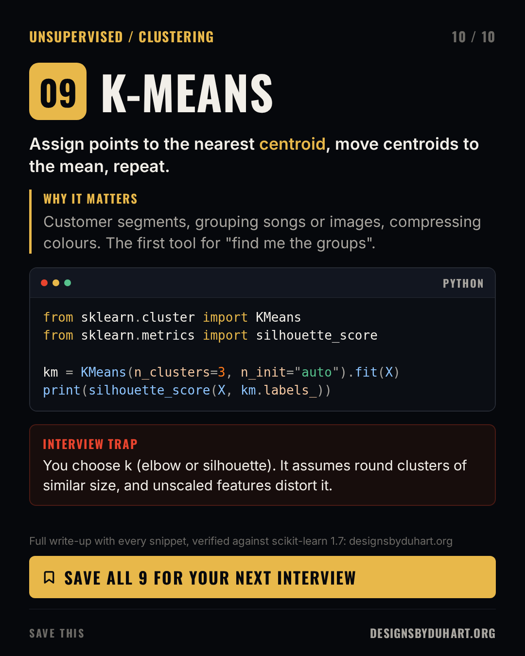
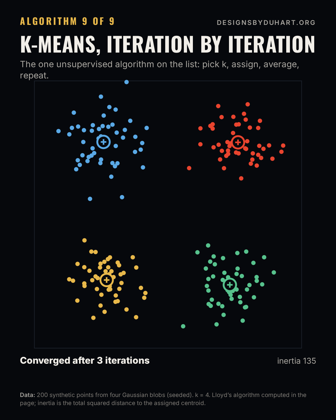
k-means is the one unsupervised algorithm on the list. Pick k, place k centroids, assign every point to its nearest centroid, move each centroid to the mean of its points, and repeat until nothing changes. It's fast and simple and it's the first thing to try when someone says "find the groups": customer segments, similar tracks, colour palettes.
Everything about it depends on choices you make. You choose k; the elbow plot and the silhouette score help, but domain sense matters more. It assumes clusters are roughly round and similar in size, so long thin or very uneven clusters get split badly (DBSCAN or Gaussian mixtures handle those). Distances again mean you scale first. And it can converge to a poor local optimum, which is why scikit-learn uses k-means++ initialisation by default and can run several initialisations.
k-means
K-means, animated
How I choose
A rough order I follow on a new tabular problem:
- A linear or logistic regression baseline with scaled features. It tells me how much signal there is and gives me something to explain.
- Gradient boosted trees with early stopping. Usually the best model I'll get on a table.
- A random forest if I want something robust with almost no tuning, or as a check on the boosted model.
- k-NN, Naive Bayes and SVMs for the situations they're good at: similarity lookups, small text datasets, small and wide data.
- k-means when there's no label and the question is "what groups are in here".
Here's that order as code. One loop, the same cross validation for every model, and the scaling inside a pipeline so it's learned on the training folds only:
Compare several of the nine on the same folds. Runs as is with scikit-learn 1.7; swap in your own X and y.
from sklearn.datasets import make_classification
from sklearn.model_selection import cross_val_score
from sklearn.pipeline import make_pipeline
from sklearn.preprocessing import StandardScaler
from sklearn.linear_model import LogisticRegression
from sklearn.ensemble import HistGradientBoostingClassifier, RandomForestClassifier
from sklearn.neighbors import KNeighborsClassifier
from sklearn.svm import SVC

X, y = make_classification(n_samples=1000, n_features=20, n_informative=8, random_state=0)

models = {
    "logistic": make_pipeline(StandardScaler(), LogisticRegression()),
    "boosting": HistGradientBoostingClassifier(early_stopping=True),
    "forest": RandomForestClassifier(n_estimators=200),
    "knn": make_pipeline(StandardScaler(), KNeighborsClassifier()),
    "svm": make_pipeline(StandardScaler(), SVC()),
}
for name, model in models.items():
    scores = cross_val_score(model, X, y, cv=5, scoring="roc_auc")
    print(f"{name:10s} {scores.mean():.3f} +/- {scores.std():.3f}")
Whatever you pick, the interview answer that lands is the one that connects the algorithm to the data: how many rows, what types of features, do you need probabilities, do you need to explain it. Name the trap before the interviewer does.
Next in this series: five mid tier ML concepts that come up in interviews once you know these algorithms, from the bias variance tradeoff to data leakage.
Next in the interview series: 5 mid tier ML concepts you should know for interviews, from the bias variance tradeoff to data leakage.
More: LinkedIn · Instagram. Portfolio and case studies: designsbyduhart.org.
If any of this saved you an afternoon, Buy me a coffee.