5 ML Algorithms You Should Already Know (With scikit-learn Code)
Linear regression, logistic regression, random forests, k-means and gradient boosting: the intuition, when to reach for each, the gotcha that bites, and a scikit-learn snippet for every one.
Why the classics still matter
I posted a short version of this on Instagram a while ago. This one has code for every algorithm, the gotcha I'd ask about in an interview, and a runnable script at the end.
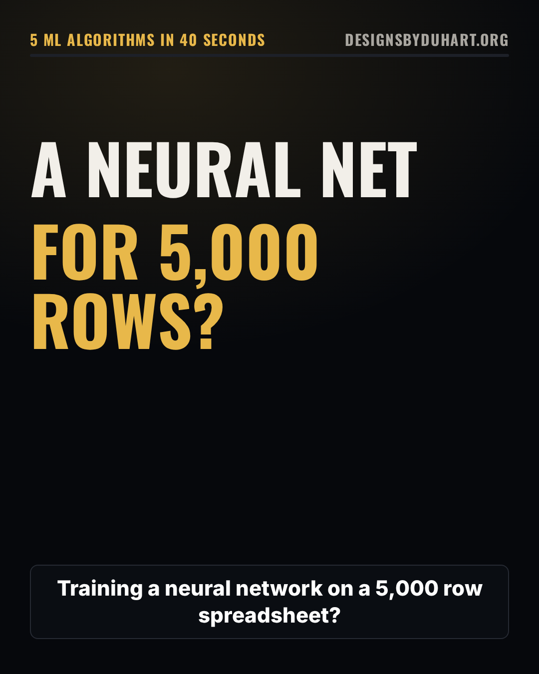
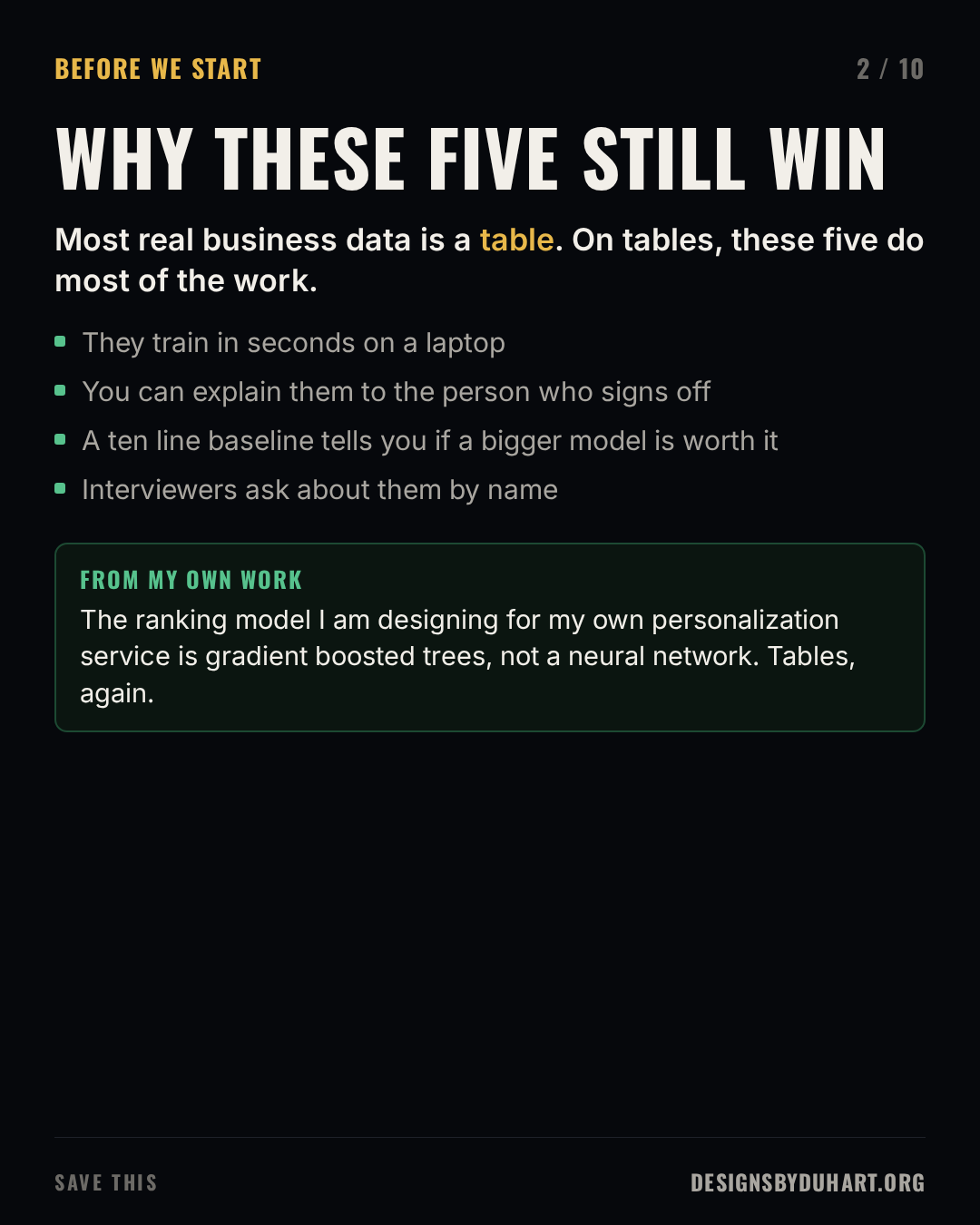
Here's the thing people skip when they jump straight to deep learning: most of the data a business owns is a table. Customers and orders, sessions and clicks, sensors and readings. On tables, five classical algorithms do most of the real work, they train in seconds, and you can explain them to the person who has to sign off on the result.
They're also the best way to find out whether you need anything bigger. A ten line baseline gives you a number. If the fancy model can't beat it by a margin that matters, you just saved yourself a GPU bill.
A personal example: the ranking model I'm designing for my own personalization service is LightGBM, which is gradient boosted trees, one model per region and product, scored inside a Go service. Not a neural network. The inputs are tables, so the classics win again.
All the snippets use scikit-learn and assume you already have X_train, X_test, y_train and y_test. The full script at the end builds those from a dataset that ships with scikit-learn, so you can run everything.
5 ML algorithms you should already know
5 ML algorithms in 40 seconds
Why these five still win
1. Linear regression
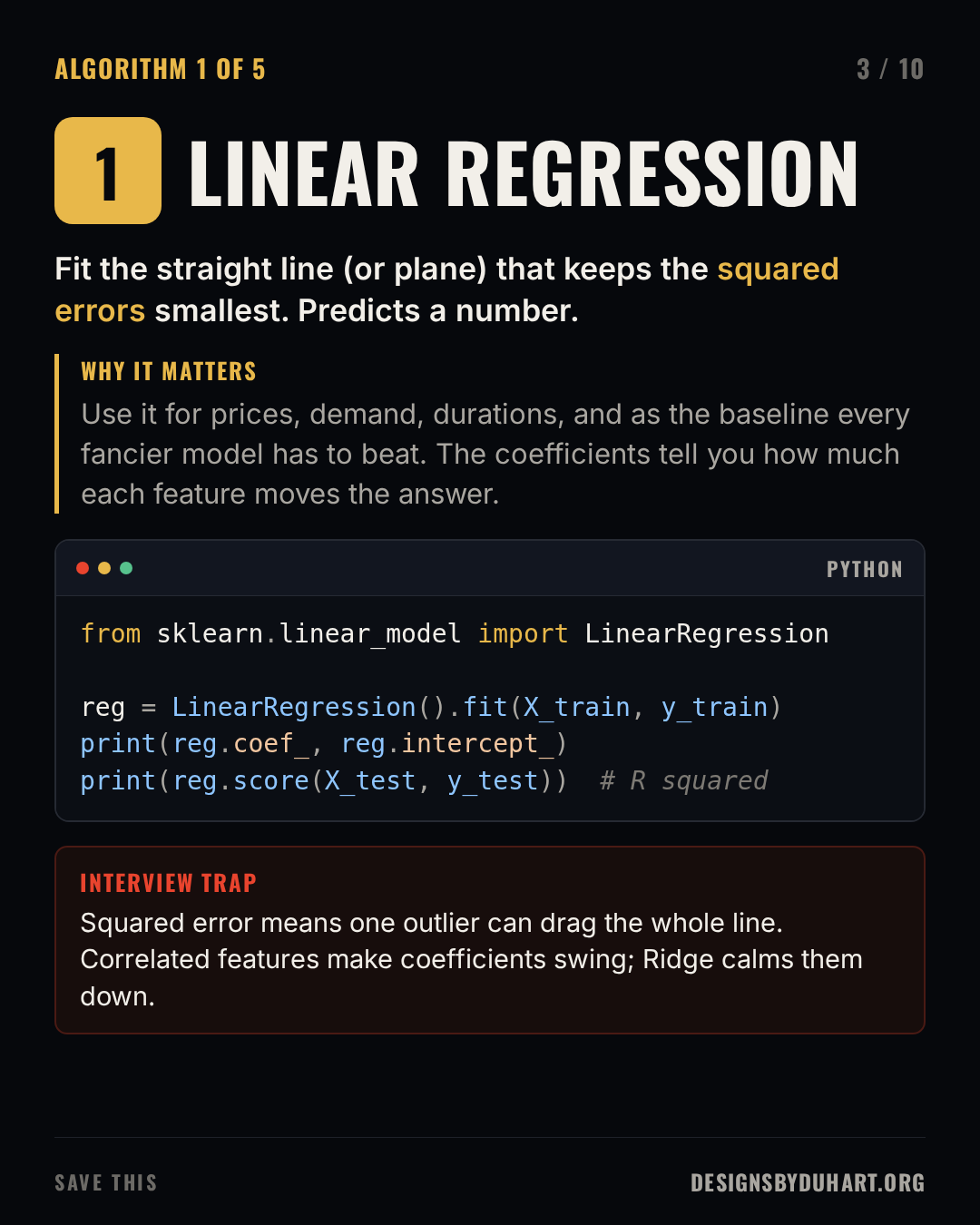
Intuition. Draw the straight line (or, with many features, the flat plane) through your data that keeps the squared distance between the line and the points as small as possible. Each feature gets a coefficient: how much the prediction moves when that feature goes up by one.
When to use it. Predicting a number: a price, a delivery time, next week's demand. And as the baseline for any regression problem, because it's fast, it's explainable, and it's surprisingly hard to beat on small, clean data.
The gotcha. Squared error punishes big misses hard, so a single outlier can pull the whole line toward it. And when two features carry the same information (square feet and number of rooms), the coefficients can swing wildly between them even though the predictions barely change. Ridge regression adds a penalty on large coefficients and calms that down.
Linear regression
2. Logistic regression
Intuition. Compute a linear score exactly like linear regression, then squeeze it through a sigmoid so it lands between 0 and 1. That number is a probability. Despite the name, it's a classifier.
When to use it. Any yes or no question: will this customer churn, is this transaction fraud, will this user click. It's the first model I'd try, because it's fast, its coefficients are readable, and you get a probability you can threshold however the business needs.
The gotcha. Two of them. First, scikit-learn's LogisticRegression is regularised by default, which means the scale of your features changes the answer. Put a StandardScaler in front of it. Second, class imbalance. If 99 percent of your rows are "not fraud", a model that always says "not fraud" is 99 percent accurate and useless. Look at precision and recall or ROC AUC, consider class_weight="balanced", and pick the decision threshold on purpose. Nothing says it has to be 0.5.
Logistic regression
![Slide 4 of 10: LOGISTIC REGRESSION. A linear score squeezed through a sigmoid into a probability. Despite the name, it classifies. Why it matters: The first thing to try for yes or no questions: churn, fraud, click. Fast, explainable, and it gives you a probability, not just a label. A code card (python) shows: clf = make_pipeline( StandardScaler(), LogisticRegression(class_weight="balanced")) clf.fit(X_train, y_train) p = clf.predict_proba(X_test)[:, 1] Interview trap: With 99% negatives, a model that always says no is 99% accurate. Use precision, recall or ROC AUC, and pick the threshold. 0.5 is not sacred.](https://media.designsbyduhart.org/viral/89234b8ad4299729.png)
3. Decision trees and random forests
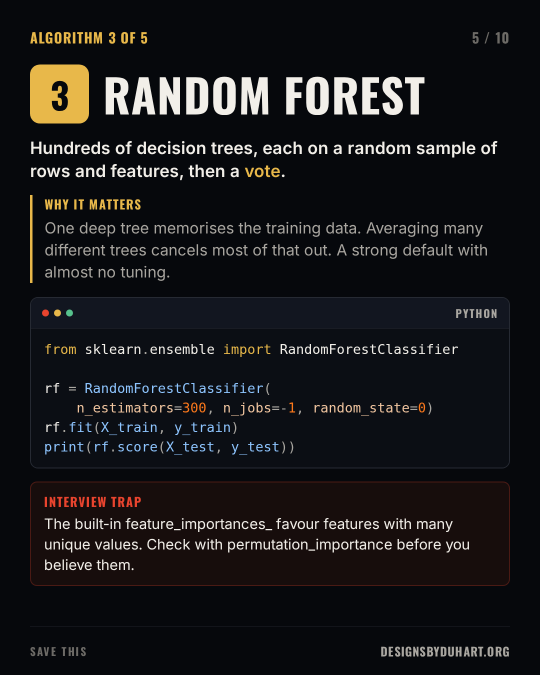
Intuition. A decision tree asks a series of yes or no questions about the features ("is income above 40k?") until it reaches an answer. One deep tree can memorise the training data perfectly and generalise badly. A random forest trains hundreds of trees, each on a random sample of the rows and a random subset of the features at every split, and lets them vote. Their individual mistakes are different, so averaging cancels most of them out.
When to use it. When you want a strong model on tabular data with almost no tuning. Forests handle non-linear relationships and interactions between features, they don't need scaled inputs, and the defaults are usually fine.
The gotcha. The built-in feature_importances_ are computed from how much each feature reduced impurity during training, and they're biased toward features with many unique values, like IDs or exact timestamps. Before you tell anyone "feature X matters most", check with permutation_importance on held-out data.
Random forest
4. K-means
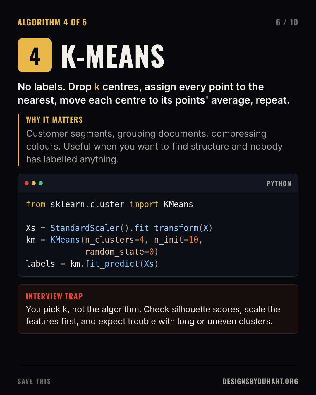
Intuition. You have no labels, just points. Pick a number k. Drop k centres, assign every point to its nearest centre, move each centre to the average of its points, and repeat until nothing moves. What you get is k groups of points that are close to each other.
When to use it. Customer segmentation, grouping similar documents, reducing an image to a handful of colours. Anywhere you want to discover structure that nobody labelled.
The gotcha. The algorithm doesn't choose k. You do, so try several and compare them with silhouette scores (the elbow plot is the other common method, and it's often ambiguous). Distances drive everything, so scale your features first, or the one measured in dollars will swamp the one measured in years. And k-means assumes roughly round clusters of similar size. Long, curved or very uneven groups need something like DBSCAN or a Gaussian mixture.
K-means
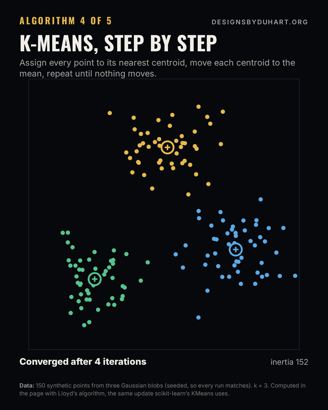
Watch k-means converge
5. Gradient boosting
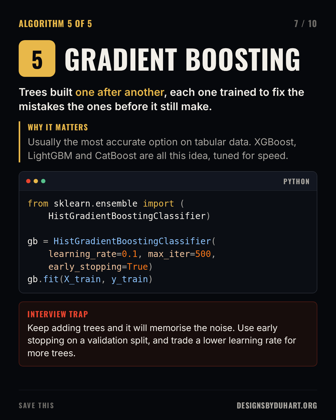
Intuition. Where a random forest builds trees independently and averages them, boosting builds them in sequence. Each new, small tree is trained on the errors the ensemble still makes (technically, on the gradient of the loss), and gets added with a small weight. Hundreds of weak trees, each correcting the last, add up to a very strong model.
When to use it. When accuracy on tabular data matters most. Gradient boosted trees win a large share of tabular competitions and run a lot of production ranking and risk systems. XGBoost, LightGBM and CatBoost are all this idea with clever engineering. In scikit-learn, HistGradientBoostingClassifier is the fast one and handles missing values natively.
The gotcha. Boosting will keep reducing training error long after it stopped learning anything real. Use early stopping on a validation split, and remember the trade: a lower learning rate needs more trees but usually generalises better.
Gradient boosting
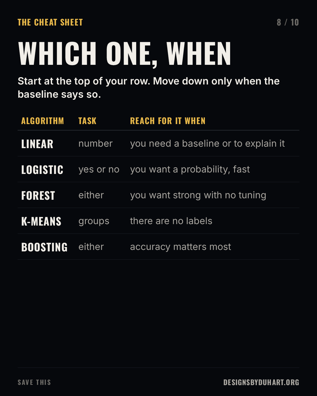
Which one, when
If you remember nothing else, remember the order. Start with the simple model for your task, get an honest score, and move down the table only when the baseline says it's worth it.
Which one, when
The trap under all five: leakage
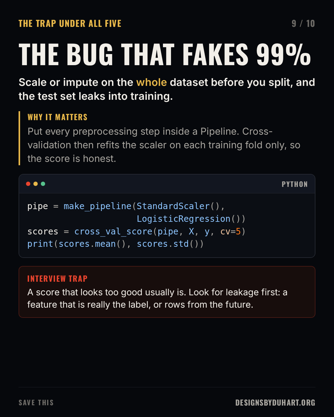
The most common way I've seen a model score 99 percent in a notebook and fall over in production is data leakage. The classic version: fit the scaler (or the imputer, or the feature selection) on the whole dataset, then split into train and test. The test set's statistics have now leaked into training, and your score is optimistic.
The fix is structural. Put every preprocessing step inside a scikit-learn Pipeline, and evaluate the pipeline with cross-validation. Each fold then refits the scaler on its own training data only. The other kind of leakage is a feature that secretly contains the answer, like a "cancellation date" column in a churn model, or rows from the future in a time series. If a score looks too good, go looking for that before you celebrate.
The bug that fakes 99%
All five on datasets that ship with scikit-learn. Runs in a few seconds on a laptop.
from sklearn.datasets import load_breast_cancer, load_diabetes
from sklearn.model_selection import train_test_split, cross_val_score
from sklearn.pipeline import make_pipeline
from sklearn.preprocessing import StandardScaler
from sklearn.linear_model import LinearRegression, LogisticRegression
from sklearn.ensemble import RandomForestClassifier, HistGradientBoostingClassifier
from sklearn.cluster import KMeans
from sklearn.metrics import roc_auc_score, silhouette_score

# regression: diabetes progression
Xr, yr = load_diabetes(return_X_y=True)
Xr_tr, Xr_te, yr_tr, yr_te = train_test_split(Xr, yr, random_state=0)
print("linear R^2", LinearRegression().fit(Xr_tr, yr_tr).score(Xr_te, yr_te))

# classification: breast cancer
X, y = load_breast_cancer(return_X_y=True)
X_tr, X_te, y_tr, y_te = train_test_split(X, y, stratify=y, random_state=0)
models = {
    "logistic": make_pipeline(StandardScaler(), LogisticRegression(max_iter=1000)),
    "forest": RandomForestClassifier(n_estimators=300, n_jobs=-1, random_state=0),
    "boosting": HistGradientBoostingClassifier(early_stopping=True, random_state=0),
}
for name, m in models.items():
    m.fit(X_tr, y_tr)
    auc = roc_auc_score(y_te, m.predict_proba(X_te)[:, 1])
    cv = cross_val_score(m, X, y, cv=5, scoring="roc_auc")
    print(f"{name:9s} test AUC {auc:.3f}  cv AUC {cv.mean():.3f} +/- {cv.std():.3f}")

# clustering: same features, no labels
Xs = StandardScaler().fit_transform(X)
for k in (2, 3, 4):
    labels = KMeans(n_clusters=k, n_init=10, random_state=0).fit_predict(Xs)
    print("k-means k =", k, "silhouette", round(silhouette_score(Xs, labels), 3))
How I'd answer in an interview
If someone asks which algorithm you'd use, the best first answer is a question about the data: how many rows, what kind of target, does it need to be explained. Then name the baseline you'd start with, the model you'd move to if it fell short, and how you'd measure it without fooling yourself. That answer shows judgement, which is what they're actually testing.
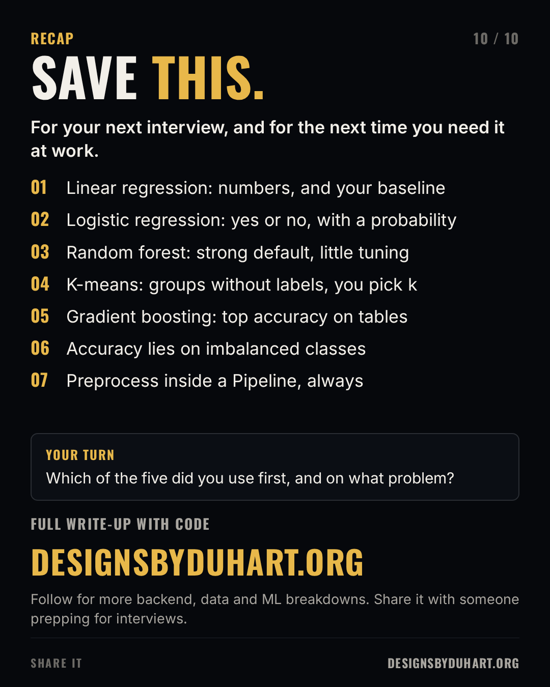
Save it for your next interview
Next in the interview series: gRPC fundamentals, from .proto contracts to streaming and load balancing.
More: LinkedIn · Instagram. Portfolio and case studies: designsbyduhart.org.
If any of this saved you an afternoon, Buy me a coffee.