Stream Wars: A New Hope for honest benchmarks? How to test a backend you can trust
The method behind One Contract, Three Runtimes: pre-registration, open-model load, chaos with a control, and what a single run cannot claim.
Episode X: A New Hope
The paper: One Contract, Three Runtimes (PDF, 24 pages)
Every Star Wars movie opens the same way. A crawl tells you where things stand before a single shot is fired. "It is a period of civil war." You know the stakes, you know the sides, and nobody can change the setup halfway through the movie.
That's how I wanted to run a benchmark, and it's the part almost nobody does.
In episode 9 I told the results of FeedBench: the hot path of my social feed built three times, as the production TypeScript on Cloudflare Workers, a Go port and a Spring Boot port, then loaded until they broke and hit with six faults. The database broke first, Go won on cost and recovery, and two indexes did more than any runtime. This episode is the other half. It's how I ran the test, what nearly sank it, and what you should copy if you want numbers you'd defend in a design review. The study is the worked example. The paper is the source for every number below.
The question, and why toy benchmarks mislead
The question was the one every backend team argues about: which runtime handles this service better at scale? The usual way to answer it is a hello world handler or a single SELECT, hit as hard as possible, with the average latency in a bar chart.
That measures the HTTP stack and the database driver. My feed's cost lives somewhere else: a visibility check on every read, a page assembled from three separately budgeted queries, writes inside transactions. A toy endpoint has none of that. It also stops at throughput, and nobody who runs production stops there. You want to know what happens when a replica dies, a neighbor steals your CPU, or the database gets slow while people are still scrolling.
So the study asked three questions. Under the same caps, who sustains the most traffic inside a latency objective, and at what cost? During a fault, how far does each one drift from normal, and how long does it take to come back? And which differences come from the language runtime, and which from everything around it?
Write it down before the first run
Sections 1 to 3 of the paper, the questions, the hypotheses, the metrics, the experiments and the abort rules, were written and committed on October 1 before any load ran (commit 28b39d10b). The finished paper keeps them exactly as written.
Three hypotheses went in:
- H1, mine: Workers beats Go and Spring under load because of edge caching.
- H2: each implementation holds steady state through every fault and recovers within 30 seconds.
- H0: there's no difference between them bigger than the spread between repeated runs.
Why bother? Because once you've seen results, every choice you make afterwards is suspect, including to you. Which percentile, which window, which run counts. Write them first and you can't quietly move the goalposts toward the answer you liked.
The part I'd tell anyone to copy is what comes next. Plans don't survive contact, and mine didn't. Section 3.10 of the paper, "Deviations from the pre-registered method", lists all 11 ways the study departed from the plan, each one stated rather than edited into the plan: the fault proxy's CPU cap, a sixth fault that wasn't in the plan, the ramp step sizes, the edge arm that replaced a planned production probe, the repetitions that never happened. That section did more for my credibility than any chart, and it also kept me honest while writing. Every time I wanted to tidy something, I had to write it down instead.
Sections 1 to 3 were written before any run, and are kept as written. Where the study departed from them, Section 3.10 says so.
One Contract, Three Runtimes, front matter
One contract, and proof the ports are honest
A comparison is only fair if everyone is doing the same work. The easiest way to win a benchmark is to skip the expensive part. So before writing a line of Go or Java, there was one written contract: nine routes, the schema, the wire format, the error table, the transaction boundaries of every write, and how a replica behaves on shutdown, on a slow database and on a dead one.
The visibility check is where a port would most likely cut a corner, so it gets two tests that every port has to pass before it's allowed near the load generator:
- Agreement. The check exists twice, as an SQL predicate for lists and as code for single reads. For a matrix of 4,320 fixture items over 495 viewer cases, the two forms and an independent oracle have to agree on every single case.
- Mutation. Drop any one clause of the check and at least one fixture must change its answer. If you can delete a clause and every test still passes, the tests aren't testing it.
Both tests came from the production TypeScript, and the Go and Spring ports carry their own copies. The paper is honest about the limit: these tests bound how far the logic can drift. They can't prove the ports are equally optimized. Both were written idiomatically and neither was tuned after the results came in.
Open model, or you're lying to yourself
This is the one I'd put on a poster.
Most load tools default to a closed loop: N virtual users, each sends a request, waits for the answer, then sends the next. It sounds realistic. It isn't. When the server stalls, every user is stuck waiting, so the load tool sends fewer requests during exactly the seconds that are slow. The bad moments get under-sampled and the percentiles look better than what real users felt. Gil Tene named this coordinated omission, and once you've seen it you can't unsee it in other people's charts.
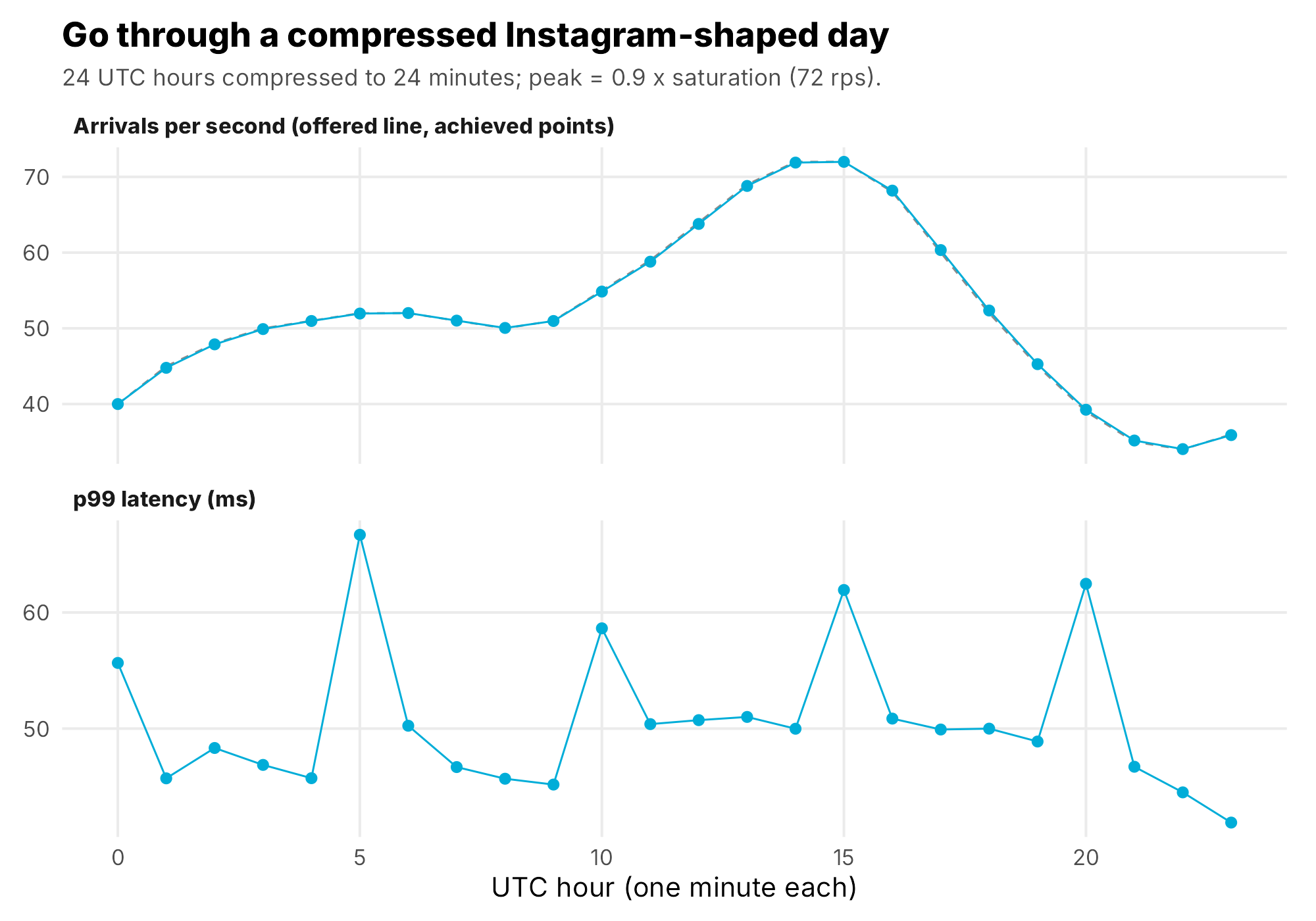
Real users don't wait for each other. They arrive on their own schedule. So every phase in FeedBench uses an open model: k6's constant-arrival-rate and ramping-arrival-rate executors start requests on the clock whether the server keeps up or not. If k6 can't start a scheduled request because every virtual user is busy, it records a dropped arrival, and the saturation rule counts drops against the contender. A server can't look fast by making the load generator wait.
The step ramp: arrival rate, not users. Each step jumps in 2 s and holds for the rest of the minute, and the run aborts itself if more than half of all requests fail after the first minute. Trimmed from harness/k6/feedbench.js.
const stages = [];
for (let r = start; r <= max; r += step) {
  stages.push({ duration: '2s', target: r }, { duration: `${stepS - 2}s`, target: r });
}
export const options = {
  scenarios: {
    control: {
      executor: 'ramping-arrival-rate', startRate: start, timeUnit: '1s',
      startTime: `${warm}s`, stages, maxVUs: MAX_VUS, exec: 'arrival',
    },
  },
  thresholds: {
    // more than half failing after a minute means down, not degraded: stop
    http_req_failed: [{ threshold: 'rate<0.5', abortOnFail: true, delayAbortEval: '60s' }],
  },
};
An open model follows its schedule
Steady state, SLO and saturation, defined from output
Chaos engineering starts from steady state, and steady state has to be something you measure from the outside: p99 latency, error rate (5xx plus requests that never got an answer) and achieved throughput. Not CPU, not queue depth, not "the dashboard looks fine". Internal gauges explain a result. They don't define one.
The objective was p99 under 500 ms and errors under 1%, over a 60 second window. Saturation is the highest step of a ramp where that holds, with no dropped arrivals, skipping the first 5 seconds of each step.
Even that sounds more precise than it is, so the paper reports saturation under five definitions side by side instead of choosing the flattering one afterwards. For Go and Spring they all agree. For local Workers they don't: 15 arrivals per second by the step rule, 10 if every single second in the step must stay under 500 ms, because one second inside the 15 step hit 560 ms. Go with its cache passes at 190 but fails at 180, so its knee is 170. If a definition can change your answer, show all of them.
Every fault then runs at 70% of each contender's own saturation: Go 56, Spring 63, Workers 10 and Go with cache 133 arrivals per second. That puts each one at the same headroom, not the same load, which matters when you read the fault results.
The chaos method: steady state, hypothesis, inject, observe
The fault experiments follow Basiri and colleagues' chaos engineering paper from Netflix. Define steady state. Hypothesize that it holds in both a control and the experiment. Inject faults that happen in the real world. Look for a difference.
The control is the part people skip. Every FeedBench fault run has the same timeline: 120 seconds of warm-up that's thrown away (the JVM needs it, the others get it for symmetry), 120 seconds of control, the fault, then 180 seconds of recovery. "p99 went up during the fault" means nothing until you know what p99 was two minutes earlier on the same system.
The six faults, each with its hypothesis written before it ran:
- Kill a replica with SIGKILL, restart it 30 seconds later.
- Graceful termination with SIGTERM, like a deploy.
- Steal the CPU with a stress-ng neighbor pinned to the replica's cores.
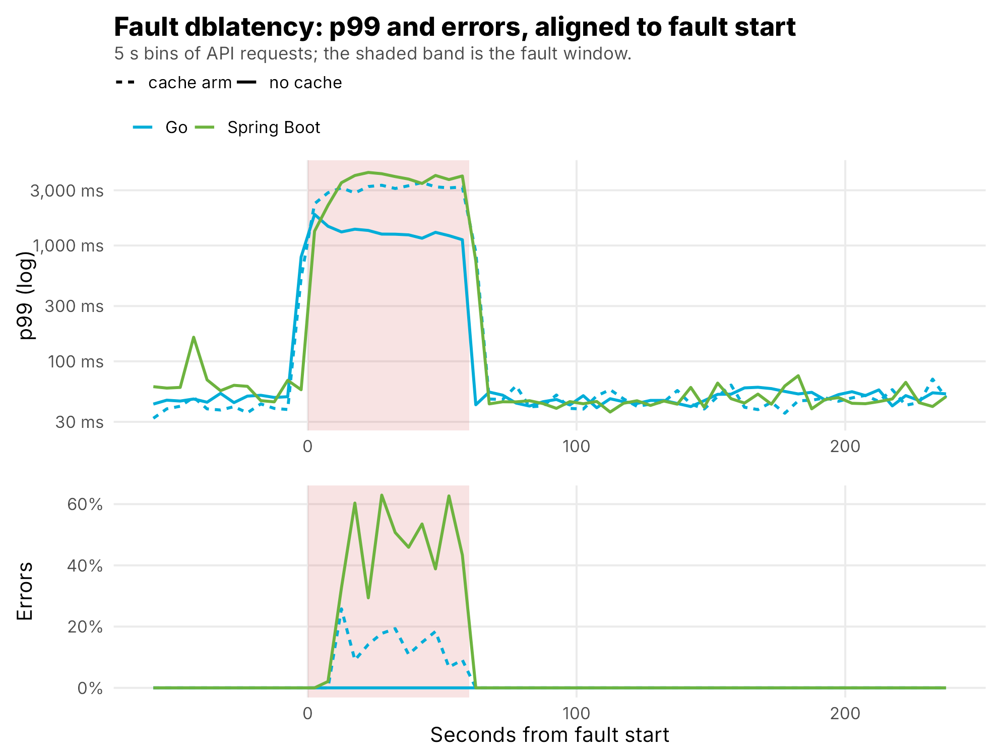
- +100 ms on every database call, with 20 ms of jitter.
- Cut the database for 15 seconds.
- +150 ms on the object store.
And abort rules, also written first: the run kills itself if the host drops below 1.5 GB of available memory, or if more than half of all requests fail. The host runs other production services, so the experiment had to be able to stop itself.
Control, fault, recovery in one picture
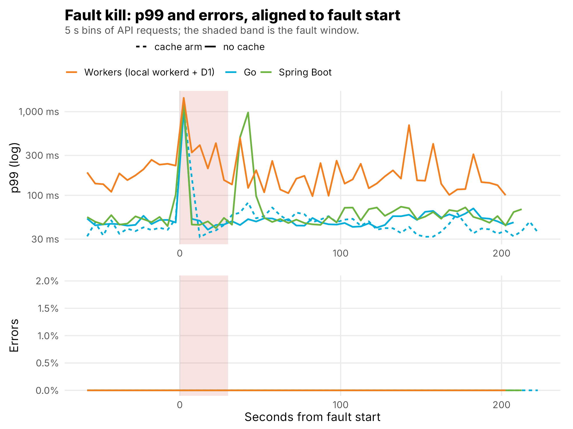
The faults also showed why you write hypotheses per experiment. For the CPU flood I predicted that nobody's health check would notice, because a SELECT 1 stays cheap, so the load balancer would keep routing to the slow replica. That's what happened. For the database latency fault I predicted the pool would run out, and it did for some: Go without cache at 56 arrivals per second absorbed it with zero errors and a 1.5 s p99, while Spring at 63 failed 41.6% of requests. The runs were at different loads, so the paper reads that as where each configuration broke, not which language is tougher.
+100 ms on the database link
The metrics that matter
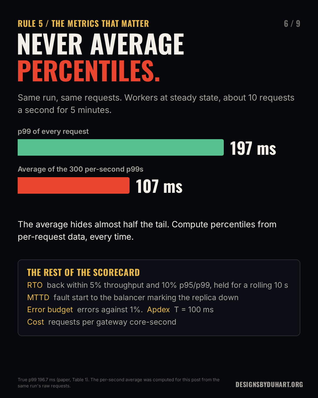
Percentiles come from every request, never from averaging percentiles. k6 logged every request with its timestamp, route, status and duration, and every percentile in the paper is computed over the raw requests in its window. The tempting shortcut is to compute a p99 per second and then average those. It's wrong, and not by a little.
Two ways to get a p99 from the same control phase. Only one is a p99.
library(data.table)
api <- fread(cmd = "gzip -dc requests.csv.gz")[kind == "api" & phase_k6 == "control"]

# Wrong: a p99 for every second, then the mean of those
avg_of_p99 <- api[, .(p99 = quantile(duration_ms, .99)), by = t_sec][, mean(p99)]

# Right: one p99 over every request in the window
p99 <- api[, quantile(duration_ms, .99)]
I ran both on the baselines for this post. For local Workers at about 10 requests a second, the true p99 is 196.7 ms. The average of the 300 per-second p99s is 107.4 ms. The shortcut hides almost half the tail. Even Go, at about 59 requests a second, drops from 59.4 to 49.1 ms. At tens of requests per second a one-second p99 is really just the slowest request in that second, and averaging those isn't any percentile at all. (I checked these in Python against the same files; the true p99s match the paper's Table 1.)
Same run, two answers
The rest of the scorecard, all defined before the first run:
- RTO, recovery time: from the fault being lifted to the start of the first 10 second window where throughput is within 5% of control and p95 and p99 are within 10%. My first version tested single seconds, and it almost never passed, because per-second throughput swings about 15% at these rates. A rolling window fixed that. When a system never recovers inside the observation window, it's reported as such, never filled in.
- MTTD, time to detect: fault start to the first 1 second HAProxy sample showing the replica down. Its resolution is the sampling interval, so it's an upper bound to about a second.
- Error budget burn: the failure rate in the fault window over a 1% budget. Cutting the database burned at 99.5 times the sustainable rate, which sounds terrible and was exactly the design, because failing fast with a 503 in 2 ms beats holding connections.
- Apdex at T = 100 ms: satisfied plus half of tolerating, over everything. One user-shaped number per phase.
- Requests per gateway core-second, integrated from the cgroup samples over their own timestamps. This is the one that separated the runtimes: Go 138, Spring 106, Workers 35.
The RTO window test, cut down to its three conditions:
The three conditions a 10 second window has to meet to count as recovered. The full function, and MTTD, are in episode 9 and in the paper's Appendix B.
recovered <- function(w, rps, ctl) {   # w: durations in one 10 s window
  abs(rps - ctl$rps) <= 0.05 * ctl$rps &&   # throughput within 5% of control
  q7(w, .95) <= 1.10 * ctl$p95 &&           # p95 within 10%
  q7(w, .99) <= 1.10 * ctl$p99              # p99 within 10%
}
One more habit: compute every number twice, independently. The harness wrote its own summary in Python, and I recomputed everything in R from the raw files. They agree on every saturation point, RTO and detection time. Where they didn't, early on, the bug was always in one of them, and once in the analysis itself: Spring's efficiency first came out NA because a sum over a per-second series with a missing sample wasn't told to skip the gap. The full R listings are in episode 9 and in Appendix B of the paper.
The threats that nearly sank it
This is the section I learned the most from. Every one of these produced numbers that looked fine.
The fault proxy capped Go and Spring. Toxiproxy sits between every gateway and its database so I can inject latency and outages. The plan said 0.25 CPU. It ran at 0.5 CPU and 128 MB, and at that cap it was pinned at 100% in every early Go and Spring run. Those runs all "saturated near 80 arrivals per second, Postgres-bound". Clean, plausible, wrong. When the proxy ran out of memory in the cache runs, the gateways logged hostname resolution errors, which sent me looking in the wrong place. I only found it by reading the proxy's own CPU in the container stats. 22 run directories went to _invalid_toxiproxy_cap/ and everything was rerun with the proxy at 2 CPU and 512 MB, where it peaked at 23% at 150 arrivals per second. Go and Spring saturated near 80 to 90 again afterwards, and the paper calls that a coincidence of this testbed, not a confirmation of the bad runs. Now every analysed run reports the p95 CPU of k6, the proxy, HAProxy and the object store.
k6 ran out of memory. Above about 700 virtual users at 2 GB, k6 was OOM-killed: 724 allocated VUs in 2,080 MB, about 2.87 MB each. So the VU cap is derived from that measurement instead of guessed. Past the cap, k6 records dropped arrivals, which count against the contender, so the cap can't hide latency either. Even so, k6 hit 100% of its memory far up every Go and Spring ramp, past every saturation point. That far end is load-generator-limited and isn't used for any result.
The VU cap, from a measured ratio instead of a guess. From harness/run.sh.
# k6 was OOM-killed holding 724 allocated VUs in 2,080 MB: 2.87 MB per VU.
# Cap = k6 memory x 0.8 headroom / 2.87 MB. At this host's 2 GB cap that is 570.
VU_MB="${VU_MB:-2.87}"
max_vus() {
  local m="${CAP_K6_MEM:-2g}" mb
  case "$m" in *g|*G) mb=$(( ${m%[gG]} * 1024 ));; *m|*M) mb=${m%[mM]};; *) mb=$(( m / 1048576 ));; esac
  python3 -c "print(int($mb*0.8/$VU_MB))"
}
The part of the chart you shouldn't read
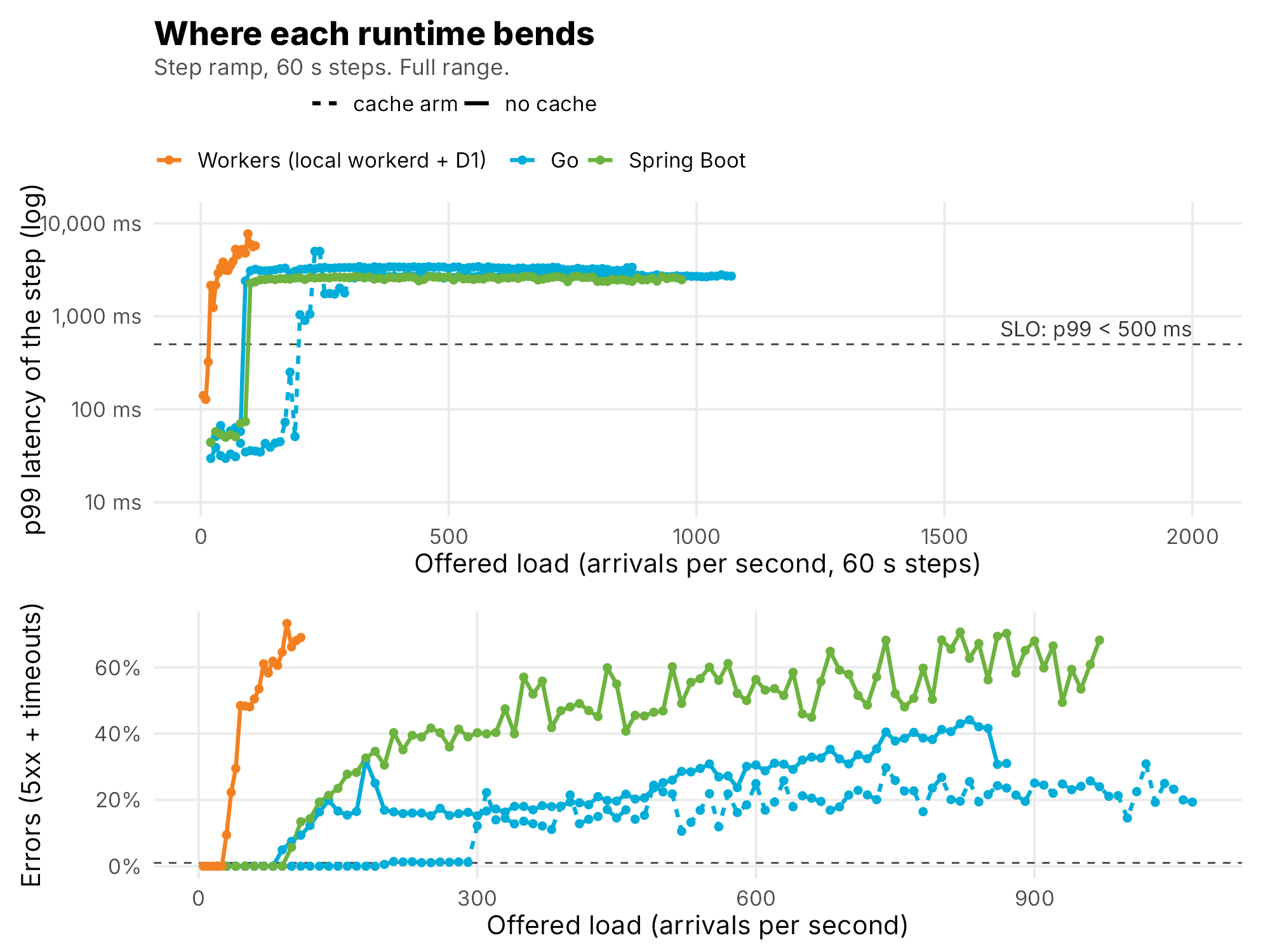
The baseline-rate bug. A default ran two baselines at a fixed 100 arrivals per second instead of 70% of each contender's saturation. Both were thrown out and rerun. A default is a decision you didn't know you made.
The disk filled up. Uploaded test media piled up to 57 GB in the object store and filled the disk at about 04:15 UTC on October 2. Postgres started failing checkpoints. 52 run directories from after that point were excluded, including every second and third repetition. Teardown now deletes the upload prefixes.
Someone else pruned every image. On October 3 an unrelated session on the same host ran a host-wide Docker prune and removed the gateway images mid-study. I rebuilt them from unchanged source. One analysed Spring run used the rebuilt image, and the paper flags it, because identical source doesn't guarantee identical binaries. The rule I took from it: never prune on a shared host.
Single runs. All of the above ate the repetitions. Three runs per configuration were planned. Only the first pass completed.
The first thing to measure in a benchmark is the benchmark.
One Contract, Three Runtimes, section 7
What the paper can and cannot claim
H0 cannot be rejected. H0 compares differences against the spread between repeated runs, and that spread was never measured. Every number is one run: 30 local configurations and 4 on the edge, with 27 planned configurations not run. So the paper calls no difference significant.
There are bootstrap intervals for the baselines, for example Go over Spring p99 at 0.873 [0.844, 0.910]. They look rigorous. They describe sampling noise inside one run, and on a shared host the run-to-run term is probably the bigger one. They're reported as descriptions, not tests.
What it can say is narrower and still useful. Some gaps are far bigger than any plausible noise: two Go replicas in 28 MB against 594 MB for Spring, 0.4 s against 18 s to recover from a kill, two indexes taking Go from 4 to 80 arrivals per second. H1 was partly supported: edge caching helped Workers without beating Go or Spring on this workload. H2 held for graceful termination and CPU theft in most cases and failed on latency during kills and database faults. Small gaps, like Go against Spring at steady state, are observations. The gaps that didn't run are listed as gaps, and nothing is imputed for them.
That's the line I'd want every benchmark post to draw, mine included: here's what we measured, here's what we didn't, here's what we can't tell yet.
How to reproduce it
Everything lives in the FeedBench folder of my monorepo: contract/ (the contract, schema, tuned indexes and index study), the three gateways, harness/ (runner, k6 script, chaos, monitor, summarizer, edge scripts), results/ with the raw data, and analysis/R/, which produces every number in the paper. Appendix A of the paper lists every version and image digest. The core of a run:
From the paper's Appendix A. One contender at a time, caps on every container, then the R analysis in a capped container.
cd FeedBench/harness
./run.sh media && ./run.sh workers seed && ./run.sh go seed      # once
./run.sh go ramp     --arm nocache --schema tuned --run-id p1     # RAMP_START=20 RAMP_STEP=10
./run.sh go baseline --arm nocache --schema tuned --run-id p1 --duration 300
./run.sh go kill     --arm nocache --schema tuned --run-id p1     # term cpu dblatency dbout objlatency

cd ..
docker run --rm --cpus 1 --memory 3g -v "$PWD":/fb -w /fb rocker/tidyverse:4.4 \
  Rscript analysis/R/run_all.R
If you run it, run it three times. That's the one thing I couldn't do.
The checklist
- Write the questions, hypotheses, metrics and abort rules before the first run. Keep a deviations section and use it.
- Give every contender one contract, and prove they follow it before you time them.
- Use an open model. Count what the load generator couldn't send against the server.
- Define steady state, the SLO and saturation from output, and show every definition that could change the answer.
- Run every fault against a control, at the same headroom.
- Compute percentiles from every request. Never average them. Judge recovery over a window, not a second.
- Check the CPU and memory of everything in the measurement path before you believe a ceiling.
- Say what one run can't claim.
Read the full paper: One Contract, Three Runtimes (PDF). The results story is episode 9.
Next episode opens a new season. Episode 11 is Intro to Metrics, and the Metrics season takes its cue from Scarface: the world is yours, if you can count it.
Next: Intro to Metrics, episode 11 and the start of the Metrics season (Scarface). The world is yours, if you can count it.
More: LinkedIn · Instagram. Portfolio and case studies: designsbyduhart.org.
If any of this saved you an afternoon, Buy me a coffee.